
Day 29 of 30 days of Data Analytics with Projects Series — Regression( Part 2 )
Welcome back peep. Hope all’s well. This is Day 29 of 30 days of data analytics where we will be covering Regression ( Part 2).
1.Linear Regression
2. Multi Linear Regression
3. Polynomial Regression
Part 2
4. Support Vector Regression
5. Decision Tree Regression
6. Random Forest Regression
7.Project
Let’s cover the most important concepts in brief —
- Linear Regression: a statistical method used to analyze the relationship between one dependent variable and one or more independent variables by fitting a linear equation to the observed data.
- Multi Linear Regression: a statistical method used to analyze the relationship between one dependent variable and two or more independent variables by fitting a linear equation to the observed data.
- Polynomial Regression: a form of regression analysis in which the relationship between the independent variable x and the dependent variable y is modeled as an nth degree polynomial.
- Support Vector Regression: a type of support vector machine that is used for regression problems. It uses the same basic idea as SVM for classification, but the algorithm is adapted for regression.
- Decision Tree Regression: a type of decision tree used for regression problems. It creates a model that predicts a value for a given input.
- Random Forest Regression: a type of ensemble learning method for regression problems, where a number of decision trees are created and combined to make a final prediction.
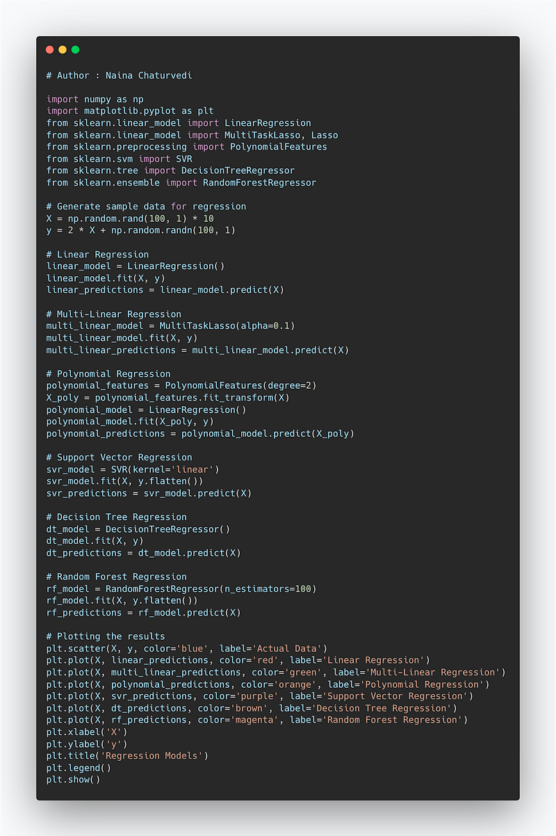
Example Code Implementation —
import numpy as np
import matplotlib.pyplot as plt
from sklearn.linear_model import LinearRegression
from sklearn.linear_model import MultiTaskLasso, Lasso
from sklearn.preprocessing import PolynomialFeatures
from sklearn.svm import SVR
from sklearn.tree import DecisionTreeRegressor
from sklearn.ensemble import RandomForestRegressor

# Generate sample data for regression
X = np.random.rand(100, 1) * 10
y = 2 * X + np.random.randn(100, 1)

# Linear Regression
linear_model = LinearRegression()
linear_model.fit(X, y)
linear_predictions = linear_model.predict(X)

# Multi-Linear Regression
multi_linear_model = MultiTaskLasso(alpha=0.1)
multi_linear_model.fit(X, y)
multi_linear_predictions = multi_linear_model.predict(X)

# Polynomial Regression
polynomial_features = PolynomialFeatures(degree=2)
X_poly = polynomial_features.fit_transform(X)
polynomial_model = LinearRegression()
polynomial_model.fit(X_poly, y)
polynomial_predictions = polynomial_model.predict(X_poly)

# Support Vector Regression
svr_model = SVR(kernel='linear')
svr_model.fit(X, y.flatten())
svr_predictions = svr_model.predict(X)

# Decision Tree Regression
dt_model = DecisionTreeRegressor()
dt_model.fit(X, y)
dt_predictions = dt_model.predict(X)

# Random Forest Regression
rf_model = RandomForestRegressor(n_estimators=100)
rf_model.fit(X, y.flatten())
rf_predictions = rf_model.predict(X)

# Plotting the results
plt.scatter(X, y, color='blue', label='Actual Data')
plt.plot(X, linear_predictions, color='red', label='Linear Regression')
plt.plot(X, multi_linear_predictions, color='green', label='Multi-Linear Regression')
plt.plot(X, polynomial_predictions, color='orange', label='Polynomial Regression')
plt.plot(X, svr_predictions, color='purple', label='Support Vector Regression')
plt.plot(X, dt_predictions, color='brown', label='Decision Tree Regression')
plt.plot(X, rf_predictions, color='magenta', label='Random Forest Regression')
plt.xlabel('X')
plt.ylabel('y')
plt.title('Regression Models')
plt.legend()
plt.show()- Linear Regression: We use the
LinearRegressionclass from scikit-learn to fit a linear equation to the data and predict the values. - Multi-Linear Regression: We use the
MultiTaskLassoclass from scikit-learn to fit a linear equation with multiple targets (in this case, only one target) and predict the values. - Polynomial Regression: We use the
PolynomialFeaturesclass to transform the original features into polynomial features, and then fit a linear equation usingLinearRegressionto predict the values. - Support Vector Regression: We use the
SVRclass from scikit-learn to perform Support Vector Regression with a linear kernel and predict the values. - Decision Tree Regression: We use the
DecisionTreeRegressorclass from scikit-learn to fit a decision tree model and predict the values. - Random Forest Regression: We use the
RandomForestRegressorclass from scikit-learn to fit an ensemble of decision trees and predict the values.
Snippet —
What’s covered in 30 days of Data Analytics Series till now —
Day 1 : Data Analytics basics and kickstart of Data analytics with projects series
Day 3 : Data Analytics Ecosystem — Data Life Cycle, Data Analysis complete process ( most important things)
Day 5 : Statistics
Day 6 : Basic and Advanced SQL
Day 8 : Pandas and Numpy
Day 9 : Data Manipulation
Day 10 : Data Visualization — Part 1
Day 11 : Project 1 : Data Visualization — Part 2
Day 12 : Data Visualization — Part 3
Day 13: Tableau — Part 1
Day 14: Tableau — Part 2
Day 15: Tableau — Part 3
Day 16 : Data Analysis Project 2
Day 17 : Data Analysis Project 3
Day 18: Data Analysis Project 4
Day 20 : Data Analysis Project 6
Day 21 : Data Analysis Project 7
Take Complete Hands On Tableau Course : Link
Projects Videos —
All the projects, data structures, SQL, algorithms, system design, Data Science and ML , Data Analytics, Data Engineering, , Implemented Data Science and ML projects, Implemented Data Engineering Projects, Implemented Deep Learning Projects, Implemented Machine Learning Ops Projects, Implemented Time Series Analysis and Forecasting Projects, Implemented Applied Machine Learning Projects, Implemented Tensorflow and Keras Projects, Implemented PyTorch Projects, Implemented Scikit Learn Projects, Implemented Big Data Projects, Implemented Cloud Machine Learning Projects, Implemented Neural Networks Projects, Implemented OpenCV Projects,Complete ML Research Papers Summarized, Implemented Data Analytics projects, Implemented Data Visualization Projects, Implemented Data Mining Projects, Implemented Natural Leaning Processing Projects, MLOps and Deep Learning, Applied Machine Learning with Projects Series, PyTorch with Projects Series, Tensorflow and Keras with Projects Series, Scikit Learn Series with Projects, Time Series Analysis and Forecasting with Projects Series, ML System Design Case Studies Series videos will be published on our youtube channel ( just launched).
Subscribe today!
Tech Newsletter —
If you are interested, you can join my newsletter through which I send tech interview tips, techniques, patterns, hacks — Software Development, ML, Data Science, Startups and Technology projects to more than 30K readers. You can subscribe to Tech Brew :
Let’s get started with the part 2!
Support Vector Regression
The Linear Regression method is basically a linear approach for modeling the relationship between a scalar dependent variable y and one or more explanatory variables (or independent variables) as it just minimizes the least squares error: for one object target y = x^T * w, where w is model’s weights.
Loss(w) = Sum_1_N(x_n^T * w — y_n) ^ 2 → min(w)
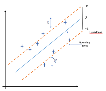
In this, we try to minimize the errors between the prediction and data. In Support Vector Regression (SVR) the goal is that the errors do not exceed the threshold and it uses the same concept as SVM, instead for the regression problems. It supports the presence of non-linearity in the data and provides an efficient prediction model.
Two most important features of Support Vector Regression:
- Maximum margin
- Hyperplane
To build a SVR:
- Collect a training set and choose a kernel and it’s parameters
- Define the correlation matrix.
- Train and figure out the contraction coefficients to create an estimator.
- Compute the correlation vector.
from sklearn.svm import SVR
regressor = SVR(kernel = 'rbf')
regressor.fit(X, y)
y_pred = regressor.predict(3.7)
y_pred = ss_y.inverse_transform(y_pred)
where kernel can be linear, Gaussian etc.
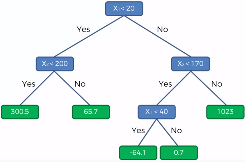
Decision Tree Regression
Decision Tree are widely used in both in classification and regression problems. These are basically predictive models that use binary rules to calculate an output/target value. Each tree has branches, nodes and leaves where the root node represents the entire population or sample.
Here is the great resource to study how does it work.
from sklearn.tree import DecisionTreeRegressor
regressor = DecisionTreeRegressor(random_state = 0)
regressor.fit(X, y)
y_pred = regressor.predict(6.5)
Random Forest Regression
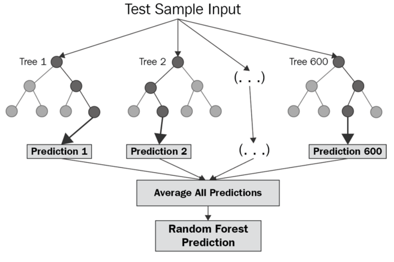
It’s a supervised machine learning algorithm that is constructed from decision tree algorithms ( it predicts the outcome by taking the average or mean of the output from the different trees) and Is used to solve both regression and classification problems. It mainly used ensemble learning, a technique in which many classifiers are combined together to provide solutions to complex problems. It’s very efficient as it reduces the overfitting of datasets, provides an effective way of handling missing data, runs efficiently on large databases, achieves extremely high accuracies, increases precision and scales really well when new features are added to the dataset..
It works well with both categorical and numerical input variables, which in-turn minimizes the time spent on one-hot encoding or labeling data.
from sklearn.ensemble import RandomForestRegressor
regressor = RandomForestRegressor(n_estimators=10, random_state=0)    regressor.fit(X, y)
y_pred = regressor.predict(4.2)
Project
Let’s dive in!
Load the data
import pandas as pd
import seaborn as sns
from matplotlib import pyplot as plt
import numpy as np
main_file_path = '../path to file/data.csv'
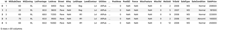
Iowadata = pd.read_csv(main_file_path)
Iowadata.head()Output —
Get to know your Data better
# Get details about your data
Iowadata.info()
Output —
<class 'pandas.core.frame.DataFrame'>
RangeIndex: 1460 entries, 0 to 1459
Data columns (total 81 columns):
Id               1460 non-null int64
MSSubClass       1460 non-null int64
MSZoning         1460 non-null object
LotFrontage      1201 non-null float64
LotArea          1460 non-null int64
Street           1460 non-null object
Alley            91 non-null object
LotShape         1460 non-null object
LandContour      1460 non-null object
Utilities        1460 non-null object
LotConfig        1460 non-null object
LandSlope        1460 non-null object
Neighborhood     1460 non-null object
Condition1       1460 non-null object
Condition2       1460 non-null object
BldgType         1460 non-null object
HouseStyle       1460 non-null object
OverallQual      1460 non-null int64
OverallCond      1460 non-null int64
YearBuilt        1460 non-null int64
YearRemodAdd     1460 non-null int64
RoofStyle        1460 non-null object
RoofMatl         1460 non-null object
Exterior1st      1460 non-null object
Exterior2nd      1460 non-null object
MasVnrType       1452 non-null object
MasVnrArea       1452 non-null float64
ExterQual        1460 non-null object
ExterCond        1460 non-null object
Foundation       1460 non-null object
BsmtQual         1423 non-null object
BsmtCond         1423 non-null object
BsmtExposure     1422 non-null object
BsmtFinType1     1423 non-null object
BsmtFinSF1       1460 non-null int64
BsmtFinType2     1422 non-null object
BsmtFinSF2       1460 non-null int64
BsmtUnfSF        1460 non-null int64
TotalBsmtSF      1460 non-null int64
Heating          1460 non-null object
HeatingQC        1460 non-null object
CentralAir       1460 non-null object
Electrical       1459 non-null object
1stFlrSF         1460 non-null int64
2ndFlrSF         1460 non-null int64
LowQualFinSF     1460 non-null int64
GrLivArea        1460 non-null int64
BsmtFullBath     1460 non-null int64
BsmtHalfBath     1460 non-null int64
FullBath         1460 non-null int64
HalfBath         1460 non-null int64
BedroomAbvGr     1460 non-null int64
KitchenAbvGr     1460 non-null int64
KitchenQual      1460 non-null object
TotRmsAbvGrd     1460 non-null int64
Functional       1460 non-null object
Fireplaces       1460 non-null int64
FireplaceQu      770 non-null object
GarageType       1379 non-null object
GarageYrBlt      1379 non-null float64
GarageFinish     1379 non-null object
GarageCars       1460 non-null int64
GarageArea       1460 non-null int64
GarageQual       1379 non-null object
GarageCond       1379 non-null object
PavedDrive       1460 non-null object
WoodDeckSF       1460 non-null int64
OpenPorchSF      1460 non-null int64
EnclosedPorch    1460 non-null int64
3SsnPorch        1460 non-null int64
ScreenPorch      1460 non-null int64
PoolArea         1460 non-null int64
PoolQC           7 non-null object
Fence            281 non-null object
MiscFeature      54 non-null object
MiscVal          1460 non-null int64
MoSold           1460 non-null int64
YrSold           1460 non-null int64
SaleType         1460 non-null object
SaleCondition    1460 non-null object
SalePrice        1460 non-null int64
dtypes: float64(3), int64(35), object(43)
memory usage: 924.0+ KB
You can see there are many null/missing values which we need to take care of. Also see which columns ( features) we would be exploring more and finally would be using in our model.
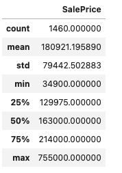
column_of_interest= ['SalePrice']
column_data=Iowadata[column_of_interest]
column_data.describe()
Output —
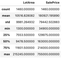
col_of_interest=['LotArea','SalePrice']
col_data=Iowadata[col_of_interest]
col_data.describe()
Output —
Data Visualization
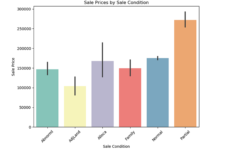
# Plot Sale Prices by Sale Condition
plt.figure(figsize=(8,6),dpi=100)sns.barplot(x=Iowadata['SaleCondition'].sort_values(ascending=True),y=Iowadata['SalePrice'].sort_values(ascending = True),data=Iowadata,orient='v',palette='Set3')
plt.title("Sale Prices by Sale Condition")
plt.xlabel('Sale Condition')
plt.ylabel('Sale Price')
plt.xticks(rotation=45)
plt.show()
Output —
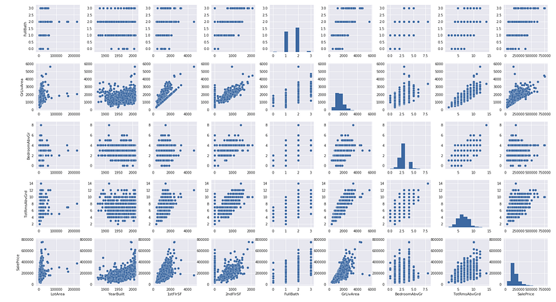
# Pair plot to Plot pairwise relationships in a datasetplt.figure(figsize=(8,6),dpi=100)
sns.pairplot(Iowadata, x_vars=["LotArea",
"YearBuilt",
"1stFlrSF",
"2ndFlrSF",
"FullBath","GrLivArea",
"BedroomAbvGr",
"TotRmsAbvGrd",'SalePrice'],y_vars=["LotArea",
"YearBuilt",
"1stFlrSF",
"2ndFlrSF",
"FullBath","GrLivArea",
"BedroomAbvGr",
"TotRmsAbvGrd",'SalePrice'] )
plt.show()Output —
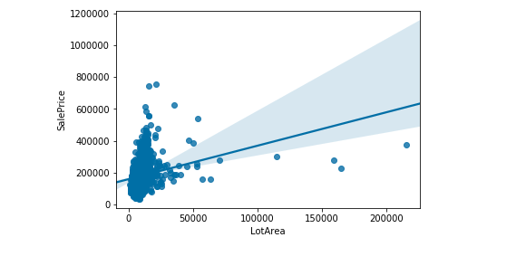
sns.regplot(data = Iowadata, x= 'LotArea',y='SalePrice' )Output —
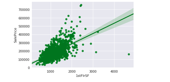
sns.regplot(data = Iowadata, x='1stFlrSF' ,y='SalePrice',color='green' )Output —
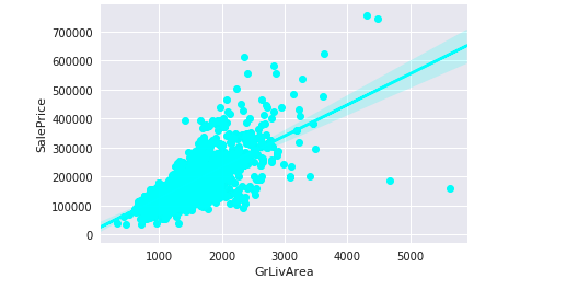
sns.regplot(data = Iowadata, x= 'GrLivArea',y='SalePrice',color='cyan' )Output —
#saleprice correlation matrixn = 10
corrmat = Iowadata.corr()
f, ax = plt.subplots(figsize=(12, 9))
cols = corrmat.nlargest(n, 'SalePrice')['SalePrice'].index
cm = np.corrcoef(Iowadata[cols].values.T)
sns.set(font_scale=1)
hm = sns.heatmap(cm, cbar=True, annot=True, square=True, fmt='.2f', annot_kws={'size': 10}, yticklabels=cols.values, xticklabels=cols.values)
plt.show()Output —
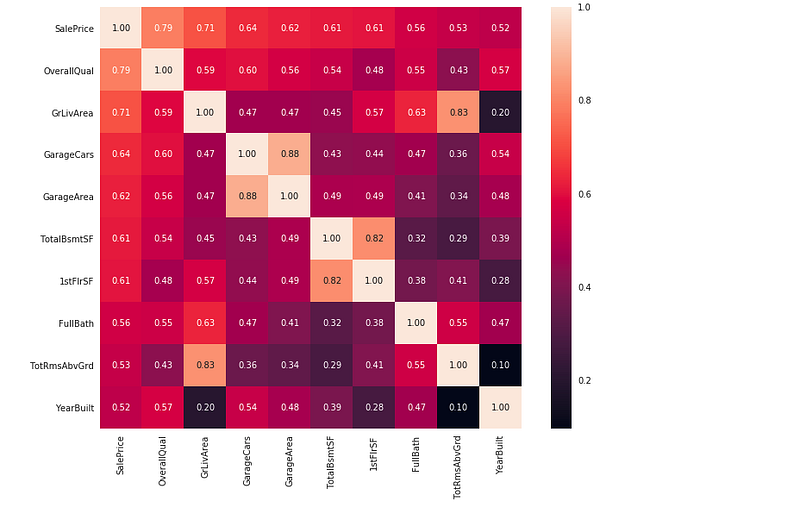
So the conclusion is ‘OverallQual’, ‘GrLivArea’ and ‘TotalBsmtSF’ are strongly correlated with ‘SalePrice’.
Decision Tree and Random Forest Regressor
from sklearn.tree import DecisionTreeRegressor
from sklearn.ensemble import RandomForestRegressor
predictor_cols = ['LotArea', 'OverallQual', 'GrLivArea','YearBuilt', 'TotRmsAbvGrd','TotalBsmtSF']# Create training predictors data
train_X = Iowadata[predictor_cols]
train_y = Iowadata.SalePriceIowa_model_d=DecisionTreeRegressor(max_depth=2) Iowa_model_d.fit(train_X,train_y)
Iowa_model_rr = RandomForestRegressor()
Iowa_model_rr.fit(train_X, train_y)
# Read the test data
test = pd.read_csv('../path to file/test.csv')
test_X = test[predictor_cols].head()
# Use the model to make predictions
predicted_prices_rr = Iowa_model_rr.predict(test_X)
predicted_prices_d = Iowa_model_d.predict(test_X)print("Predicted prices ( Decision Tree Regressor):",np.round(predicted_prices_d))
print("Predicted Prices ( RandomForest Regressor):",predicted_prices_rr)Output —
Predicted prices ( Decision Tree Regressor): [140384. 140384. 140384. 140384. 274736.]
Predicted Prices ( RandomForest Regressor): [134940. 149790. 155664. 180490. 218350.]
That’s it for now.
Find Day 30 Below:
Let me know if you have questions in the comment section below. Subscribe/ Follow, Like/Clap as it would encourage me to write more in my free time
Stay Tuned!!
Read More —
11 most important System Design Base Concepts
6. Networking, How Browsers work, Content Network Delivery ( CDN)
13. System Design Template — How to solve any System Design Question
System Design Case Studies — In Depth
Complete Data Structures and Algorithm Series
Some of the other best Series —
30 days of Data Structures and Algorithms and System Design Simplified
Data Science and Machine Learning Research ( papers) Simplified **
100 days : Your Data Science and Machine Learning Degree Series with projects
Complete Data Visualization and Pre-processing Series with projects
Exceptional Github Repos — Part 1
Exceptional Github Repos — Part 2
Tech Newsletter —
If you are interested, you can join my newsletter through which I send tech interview tips, techniques, patterns, hacks — Software Development, ML, Data Science, Startups and Technology projects to more than 30K readers. You can subscribe to Tech Brew :
For Python Projects —
For complete 60 days of Data Science and ML : Day 1 — Day 60 : Quick Recap of 60 days of Data Science and ML
Follow for more updates. Stay tuned and keep coding!
For other projects, tune to —
Build Machine Learning Pipelines( With Code)
Recurrent Neural Network with Keras
Clustering Geolocation Data in Python using DBSCAN and K-Means
Facial Expression Recognition using Keras
Hyperparameter Tuning with Keras Tuner
Custom Layers in Keras


