
Day 30 of 30 days of Data Engineering Series with Projects
Welcome back peeps to Day 30 of Data Engineering Series with Projects!
In this we will cover —
Machine Learning Algorithms
Performance metrics
Linear Regression
Logistic Regression
Decision Trees
Random Forest
Support Vector Machines
K Nearest Neighbors
K means Clustering
Hierarchical Clustering
Neural Networks
Pre-requisite to Day 30 is to complete Day 1–29( link below):
Day 3 : Complete Advanced Python for Data Engineering — Part 2
Day 18 : Data Visualization basics, Data Visualization Projects, Data Visualization using Plotly and Bokeh, Data Profiling, Summary Functions, Indexing, Grouping, Linear Regression, Multi Linear Regression, Polynomial Regression, Regression, Support Vector Regression, Decision Tree Regression, Random Forest Regression, Feature Engineering, GroupBy Features, Categorical and Numerical Features, Missing Value Analysis, Fill the missing Values, Unique Value Analysis, Univariate Analysis, Bivariate Analysis, Multivariate Analysis, Correlation Analysis, Spearman’s ρ, Pearson’s r, Kendall’s τ, Cramér’s V (φc), Phik (φk)
Day 20 : ETL ( Extract, Tranform and Load) basics, Why ETL is important?, How ETL works, ETL Tools
Day 21 : Structured Data, Semi Structured Data, Unstructured Data, Data Warehouse, Data Mart, Data Lake
Day 25: Docker, Docker vs Virtual Machines, Most important Docker commands, Kubernetes, Snowflake
Day 26 : Data Pipelines, Transformation, Processing, Workflow, Monitoring, Airflow, DAG
Day 29 : Data Engineering on cloud, AWS, AWS Services, Google Cloud Platform, GCP services
All the projects, data structures, algorithms, system design, Data Science and ML , Data Engineering, MLOps and Deep Learning videos will be published on our youtube channel ( just launched).
Subscribe today!
Tech Newsletter —
If you are interested, you can join my newsletter through which I send tech interview tips, techniques, patterns, hacks — Software Development, ML, Data Science, Startups and Technology projects to more than 30K readers. You can subscribe to Ignito:
System Design Case Studies — In Depth
Design Instagram
Design Netflix
Design Reddit
Design Amazon
Design Messenger App
Design Twitter
Design URL Shortener
Design Dropbox
Design Youtube
Design API Rate Limiter
Design Web Crawler
Design Amazon Prime Video
Design Facebook’s Newsfeed
Design Yelp
Design Uber
Design Tinder
Design Tiktok
Design Whatsapp
Most Popular System Design Questions
Mega Compilation : Solved System Design Case studies
Let’s get started!
1.Machine Learning Algorithms: These are mathematical models that are used to analyze and make predictions from data. Some popular machine learning algorithms include:
- Linear Regression: A type of supervised learning algorithm that is used for predicting continuous values.
- Logistic Regression: A type of supervised learning algorithm that is used for predicting binary outcomes.
- Decision Trees: A type of supervised learning algorithm that is used for both classification and regression problems.
- Random Forest: A type of ensemble learning algorithm that combines multiple decision trees to improve the accuracy of predictions.
- Support Vector Machines (SVMs): A type of supervised learning algorithm that is used for both classification and regression problems.
- K Nearest Neighbors (KNN): A type of supervised learning algorithm that is used for classification and regression problems.
- K-means Clustering: A type of unsupervised learning algorithm that is used for grouping similar data points together.
- Hierarchical Clustering: A type of unsupervised learning algorithm that is used to group similar data points into a hierarchical structure.
- Neural Networks: A type of supervised or unsupervised learning algorithm that is inspired by the structure and function of the human brain.
2. Performance Metrics: These are used to evaluate the performance of a machine learning model. The choice of performance metric depends on the type of problem being solved, but some common metrics include:
- Mean Absolute Error (MAE) and Mean Squared Error (MSE) for regression problems.
- Accuracy, Precision, Recall, F1 Score, AUC-ROC Curve for classification problems.
- Silhouette Score, Davies-Bouldin Index for clustering problems.
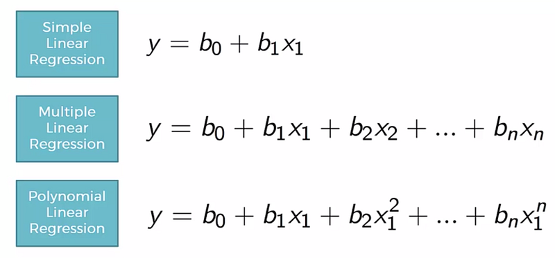
3. Linear Regression: Linear regression is a supervised learning algorithm used for predicting continuous values. It assumes a linear relationship between the input variables (also known as independent variables) and the output variable (also known as the dependent variable). Linear regression can be used for both simple and multiple regression.
4. Logistic Regression: Logistic regression is a supervised learning algorithm used for predicting binary outcomes. It models the probability of the default class using a logistic function. It is used for binary classification problem.
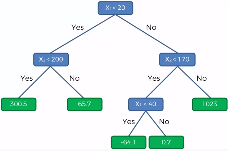
5. Decision Trees: Decision trees are a type of supervised learning algorithm that is used for both classification and regression problems. It uses a tree-like model of decisions and their possible consequences. Each internal node of the tree represents a feature(or attribute), each branch represents a decision and each leaf node represents the outcome.
6. Random Forest: Random Forest is an ensemble learning algorithm which combines multiple decision trees to improve the accuracy of predictions. It uses bagging technique and random subspace method to make decision trees more robust.
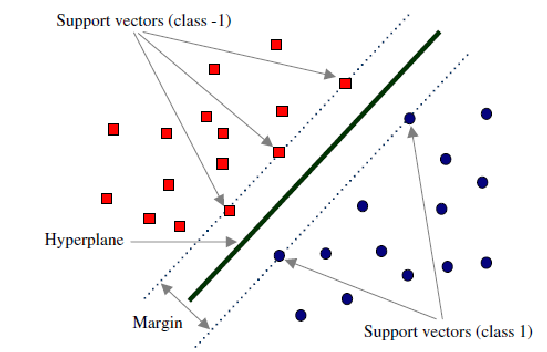
7. Support Vector Machines (SVMs): Support Vector Machines are a type of supervised learning algorithm that is used for both classification and regression problems. It tries to find a hyperplane which maximizes the margin between the different classes.
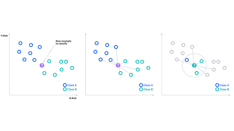
8. K Nearest Neighbors (KNN): K-nearest neighbors is a type of supervised learning algorithm that is used for classification and regression problems. It finds the k-nearest data points to a given data point, and then uses the majority class among the k-nearest points to classify the given data point.
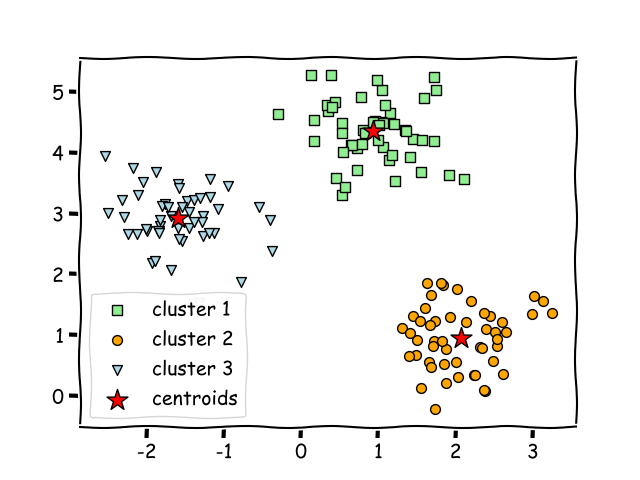
9. K-means Clustering: K-means is a type of unsupervised learning algorithm that is used for grouping similar data points together. It works by randomly initializing k centroids and then iteratively moving the centroids to the center of the data points in their cluster, while reassigning the data points to the closest centroid.
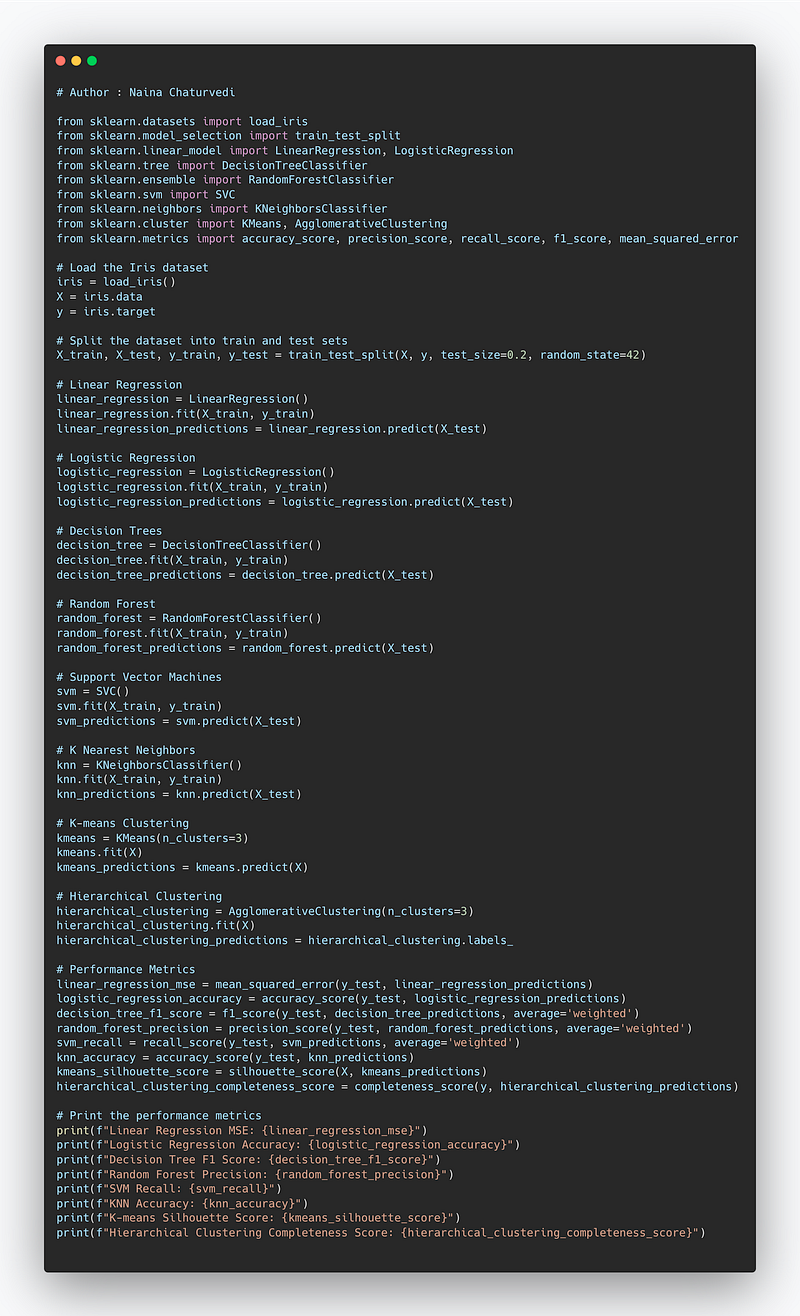
Complete Code Implementation —
from sklearn.datasets import load_iris
from sklearn.model_selection import train_test_split
from sklearn.linear_model import LinearRegression, LogisticRegression
from sklearn.tree import DecisionTreeClassifier
from sklearn.ensemble import RandomForestClassifier
from sklearn.svm import SVC
from sklearn.neighbors import KNeighborsClassifier
from sklearn.cluster import KMeans, AgglomerativeClustering
from sklearn.metrics import accuracy_score, precision_score, recall_score, f1_score, mean_squared_error

# Load the Iris dataset
iris = load_iris()
X = iris.data
y = iris.target

# Split the dataset into train and test sets
X_train, X_test, y_train, y_test = train_test_split(X, y, test_size=0.2, random_state=42)

# Linear Regression
linear_regression = LinearRegression()
linear_regression.fit(X_train, y_train)
linear_regression_predictions = linear_regression.predict(X_test)

# Logistic Regression
logistic_regression = LogisticRegression()
logistic_regression.fit(X_train, y_train)
logistic_regression_predictions = logistic_regression.predict(X_test)

# Decision Trees
decision_tree = DecisionTreeClassifier()
decision_tree.fit(X_train, y_train)
decision_tree_predictions = decision_tree.predict(X_test)

# Random Forest
random_forest = RandomForestClassifier()
random_forest.fit(X_train, y_train)
random_forest_predictions = random_forest.predict(X_test)

# Support Vector Machines
svm = SVC()
svm.fit(X_train, y_train)
svm_predictions = svm.predict(X_test)

# K Nearest Neighbors
knn = KNeighborsClassifier()
knn.fit(X_train, y_train)
knn_predictions = knn.predict(X_test)

# K-means Clustering
kmeans = KMeans(n_clusters=3)
kmeans.fit(X)
kmeans_predictions = kmeans.predict(X)

# Hierarchical Clustering
hierarchical_clustering = AgglomerativeClustering(n_clusters=3)
hierarchical_clustering.fit(X)
hierarchical_clustering_predictions = hierarchical_clustering.labels_

# Performance Metrics
linear_regression_mse = mean_squared_error(y_test, linear_regression_predictions)
logistic_regression_accuracy = accuracy_score(y_test, logistic_regression_predictions)
decision_tree_f1_score = f1_score(y_test, decision_tree_predictions, average='weighted')
random_forest_precision = precision_score(y_test, random_forest_predictions, average='weighted')
svm_recall = recall_score(y_test, svm_predictions, average='weighted')
knn_accuracy = accuracy_score(y_test, knn_predictions)
kmeans_silhouette_score = silhouette_score(X, kmeans_predictions)
hierarchical_clustering_completeness_score = completeness_score(y, hierarchical_clustering_predictions)

# Print the performance metrics
print(f"Linear Regression MSE: {linear_regression_mse}")
print(f"Logistic Regression Accuracy: {logistic_regression_accuracy}")
print(f"Decision Tree F1 Score: {decision_tree_f1_score}")
print(f"Random Forest Precision: {random_forest_precision}")
print(f"SVM Recall: {svm_recall}")
print(f"KNN Accuracy: {knn_accuracy}")
print(f"K-means Silhouette Score: {kmeans_silhouette_score}")
print(f"Hierarchical Clustering Completeness Score: {hierarchical_clustering_completeness_score}")
Snippet —
Machine Learning Algorithms
In this post we will cover the most commonly used and popular machine learning algorithms along with the code.
1. Linear Regression
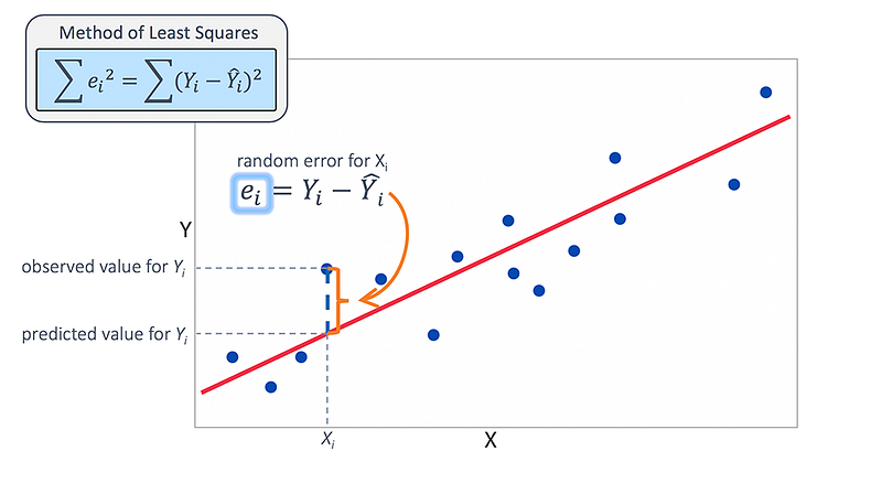
It’s a technique to estimate the relationship between two quantitative variables. It is used when you want to establish:
- Strength of the relationship — How strong the relationship is between two variables
- The value of the dependent variable at a certain value of the independent variable.
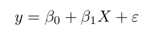
where,
y is the predicted value of the dependent variable for any given value of the independent variable which is X.
B0 is the intercept and B1 is the regression coefficient
x is the independent variable
e is the error of the estimate
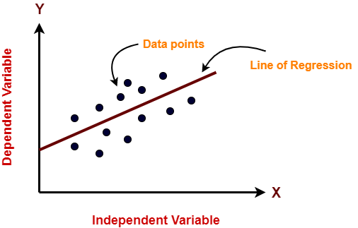
It works on the assumption that the relationship between the independent and dependent variable is linear: the line of best fit through the data points is a straight line as shown in the diagram.
In order to work with linear regression —
Import the libraries and dataset
Check for null values as well as missing data
Spilt the dataset into train and test set
Fit the dataset into the model sklearn.linear_model
Predict the result y_pred
Visualize the results using matplotlib.pyplot
from sklearn.linear_model import LinearRegression
regressor = LinearRegression()
regressor.fit(I_Train_data, D_Train_data)
preds = regressor.predict(X_test)
Visualize the training and test set
Training set results —
import matplotlib.pyplot as plt# Visualizing the Training set results
plt.scatter(X_train, y_train, color = 'green')
plt.plot(X_train, regressor.predict(X_train), color = 'blue')
plt.xlabel('Independent Variable set')
plt.ylabel('Dependent Variable set')
plt.show()Test set results —
# Visualizing the Test set results
plt.scatter(X_test, y_test, color = 'green')
plt.plot(X_train, regressor.predict(X_train), color = 'blue')
plt.xlabel('Independent Variable set')
plt.ylabel('Dependent Variable set')
plt.show()
Linear regression uses mean-square error (MSE) to calculate the error of the model. MSE is calculated by:
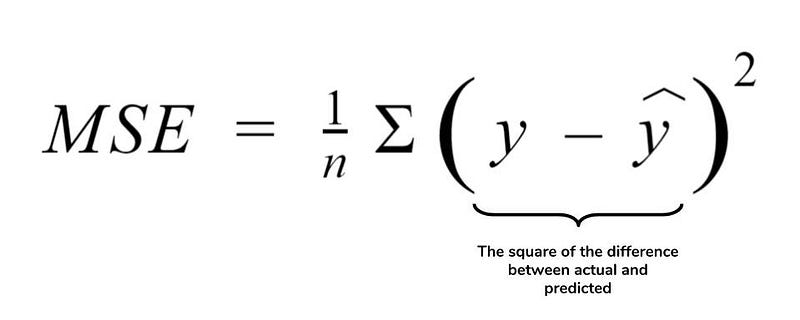
Measure the distance of the observed y-values from the predicted y-values at each value of x;
Square each of these distances and calculate the mean of each of the squared distances.
2. Multi Linear Regression
It’s used to estimate the relationship between two or more independent variables and one dependent variable. It is used when you want to establish:
- Strength of the relationship — How strong the relationship is between two or more independent variables and one dependent variable
- The value of the dependent variable at a certain value of the independent variable.
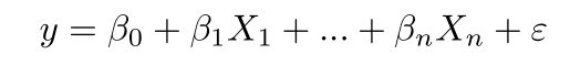
B0 = the y-intercept
B1X1= the regression coefficient (b1) of the first independent variable (x1)
BnXn = the regression coefficient of the last independent variable
y = the predicted value of the dependent variable
e = model error
Assumptions of Linear Regression
Linearity
Independence of errors
Homoscedasticity
Multivariate normality
Lack of multi collinearity
In order to find best fit line, it calculates 3 parameters —
- The t-stat of the model
- The associated p-value
- Regression coefficients
# Fitting multiple lineaar regression to the training set
from sklearn.linear_model import LinearRegression
regressor = LinearRegression()
regressor.fit(X_train, y_train)
# Predicting the test set results
y_pred = regressor.predict(X_test)X = np.append(arr = np.ones((20, 1)).astype(int), values = X, axis = 1)
X_opt = X[:, [0, 1, 2, 3, 4, 5]]
regressor_OLS = sm.OLS(endog = y, exog = X_opt).fit()
regressor_OLS.summary()
X_opt = X[:, [0, 1, 3, 4, 5]]
regressor_OLS = sm.OLS(endog=y, exog=X_opt).fit()
regressor_OLS.summary()
X_opt = X[:, [0, 3, 4, 5]]
regressor_OLS = sm.OLS(endog=y, exog=X_opt).fit()
regressor_OLS.summary()
X_opt = X[:, [0, 3, 5]]
regressor_OLS = sm.OLS(endog=y, exog=X_opt).fit()
regressor_OLS.summary()
X_opt = X[:, [0, 3]]
regressor_OLS = sm.OLS(endog=y, exog=X_opt).fit()
regressor_OLS.summary()3. Polynomial Regression
In polynomial Regression, the relationship between the independent variable x and dependent variable y is established as the nth degree polynomial providing the best approximation of the relationship between dependent and independent variables.
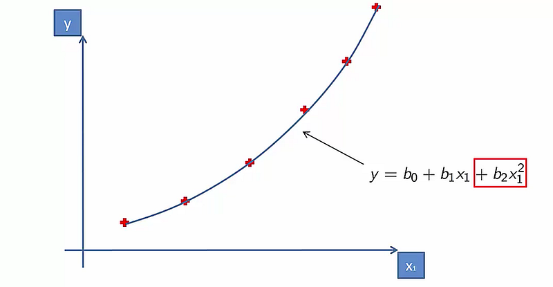
It fits a nonlinear relationship between the value of x and conditional mean of y. For cases where data points are arranged in a non-linear fashion, we need the Polynomial Regression model.
# Fitting Polynomial Regression to the datasetfrom sklearn.preprocessing import PolynomialFeatures poly = PolynomialFeatures(degree = 3) X_poly = poly.fit_transform(X) poly.fit(X_poly, y) l = LinearRegression() l.fit(X_poly, y)
4. Logistic Regression
In logistic regression, we establish the relationship between the dependent variable and one or more independent variables by estimating probabilities using an equation ( logistic regression).
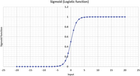
Define the Logistic Sigmoid Function 𝜎(𝑧)
def logistic_function(x):
    return 1/(1+np.exp(-x))
logistic_function(0)
Output —
0.5Compute the Cost Function 𝐽(𝜃) and Gradient
def compute_cost(theta,x,y):
    m=len(y)
    y_pred =logistic_function(np.dot(x,theta))
    error = (y * np.log(y_pred)) +(1-y) * np.log(1-y_pred)
    cost = -1/m * sum(error)
    gradient = 1/m * np.dot(x.transpose(),(y_pred - y))
    return cost[0],gradient
Cost and Gradient
mean_scores = np.mean(scores,axis=0)
std_scores = np.std(scores, axis=0)
scores = ( scores - mean_scores)/std_scores
rows = scores.shape[0]
cols = scores.shape[1]X=np.append(np.ones((rows,1)),scores,axis=1)
y=results.reshape(rows,1)theta_init = np.zeros((cols+1,1)) cost,gradient = compute_cost(theta_init,X,y)
print('Cost : ',cost)
print('Gradient : ',gradient)
Output —
Cost 0.693147180559946
Gradient
[[-0.1       ]
 [-0.28122914]
 [-0.25098615]]
Implement Gradient Descent
def gradient_descent(x,y,theta,alpha,iterations):
    costs = []
    for i in range(iterations):
        cost,gradient = compute_cost(theta,x,y)
        theta -= (alpha * gradient)
        costs.append(cost)
    return theta,costs
theta, costs = gradient_descent(X,y,theta_init,1,200)
print('Theta: ',theta)
print('Resulting Cost: ',costs[-1])
Output —
Theta
[[1.50850586]
 [3.5468762 ]
 [3.29383709]]
Resulting Cost 0.2048938203512014
Plotting the Convergence of 𝐽(𝜃)
plt.plot(costs)
plt.xlabel('Iterations')
plt.ylabel('$J(\Theta)$')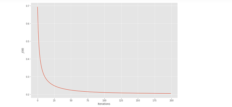
5. Decision Trees
Decision Tree are widely used in both in classification and regression problems. These are basically predictive models that use binary rules to calculate an output/target value. Each tree has branches, nodes and leaves where the root node represents the entire population or sample.
Here is the great resource to study how does it work.
from sklearn.tree import DecisionTreeRegressor
regressor = DecisionTreeRegressor(random_state = 0)
regressor.fit(X, y)
y_pred = regressor.predict(6.5)
6. Random Forest
It’s a supervised machine learning algorithm that is constructed from decision tree algorithms ( it predicts the outcome by taking the average or mean of the output from the different trees) and Is used to solve both regression and classification problems. It mainly used ensemble learning, a technique in which many classifiers are combined together to provide solutions to complex problems. It’s very efficient as it reduces the overfitting of datasets, provides an effective way of handling missing data, runs efficiently on large databases, achieves extremely high accuracies, increases precision and scales really well when new features are added to the dataset..
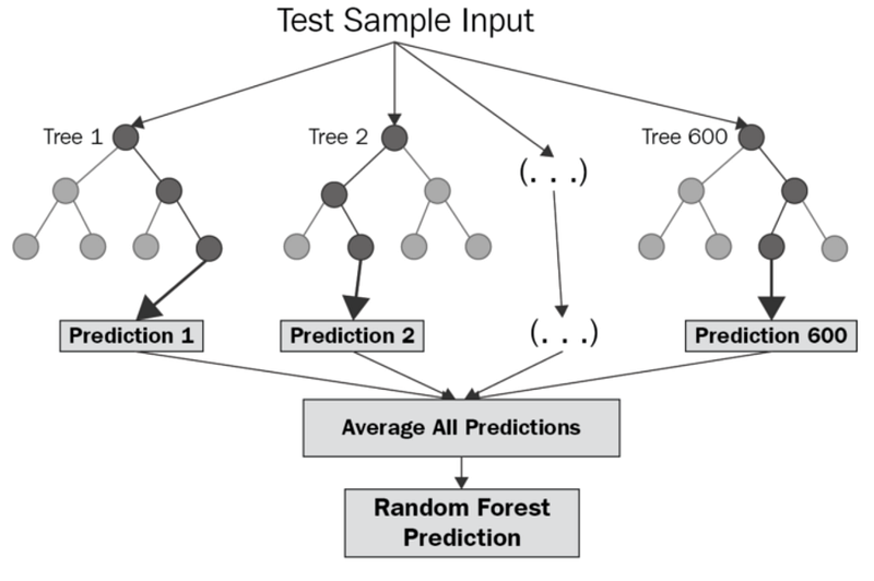
It works well with both categorical and numerical input variables, which in-turn minimizes the time spent on one-hot encoding or labeling data.
from sklearn.ensemble import RandomForestRegressor
regressor = RandomForestRegressor(n_estimators=10, random_state=0)    regressor.fit(X, y)
y_pred = regressor.predict(4.2)
7. Support Vector Machines
Support Vector Machine is a supervised machine learning algorithm which is used for both classification or regression problems. In this technique we start by plotting each data item as point in n-dimensional space with the value of a particular coordinate as being the value of the feature/independent variable. Then, we find the hyper-plane that differentiates the two classes by a boundary as shown in the image below.
Model Fitting and Predictions
svmclassifier = SVC(kernel = 'linear' , random_state = 0)
svmclassifier.fit (X_train, Y_train)
Y_pred = svmclassifier.predict(X_test)
8. K Nearest Neighbors
KNN is a classification algorithm in which the output is to predict a class membership. In order to classify an unlabeled object, the ditance of the object to the labeled object is computed, and its k nearesr neighbors are identified.
The distance measure — Euclidean distance is calculated as square root of the sum of the squared differences between a new point and an existing point.
knn = kNN()
knn.fit(X_train, y_train)
9. K means Clustering
Clustering is a technique of dividing the population or data points, grouping them into different clusters on the basis of similarity and dissimilarity between them. It helps in determining the intrinsic group among the unlabeled data points.
K-means clustering method is used and can be summarized as —
i. Divide into number of cluster K
ii. Find the centroid of the current partition
iii. Calculate the distance each points to Centroids
iv. Group based on minimum distance
v. After re-grouping/re-allotting the points, find the new centroid of the new cluster
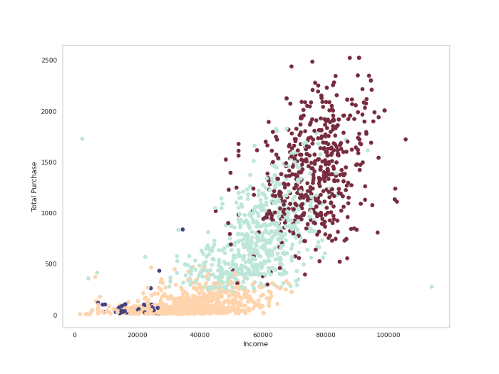
# Kmeans ( 4 Clusters )
km=KMeans(n_clusters=4,random_state=0,init="k-means++")
km.fit(c_df_final)
clusters=km.predict(c_df_final)
c_df['cluster_no'] = clusters#plotplt.figure(figsize=(12,9))
plt.scatter(df['Income'],df['Total_purchase'],c=clusters, cmap='icefire')
plt.xlabel('Income')
plt.ylabel('Total Purchase')
plt.grid(False)
plt.show()
Output —
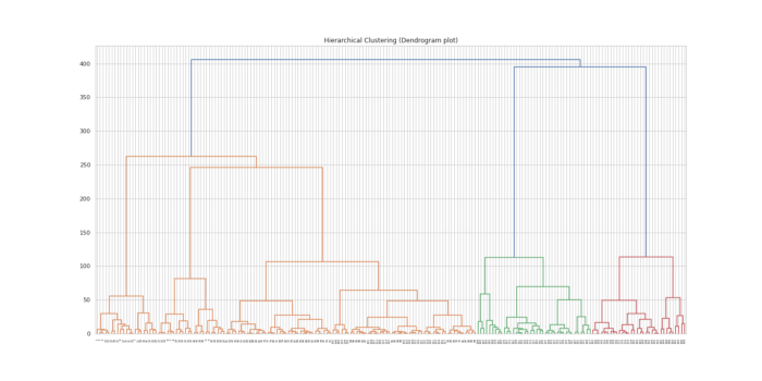
10. Hierarchical Clustering
In simple terms, the algorithm builds a hierarchy of clusters starting from the all the data points assigned to their own cluster.
The algorithm exits when there’s only single cluster is left.
There are two types of hierarchical clustering — Agglomerative hierarchical clustering and Dendrogram.
# Hierarchical Clustering ( Dendogram)
X=df.iloc[:, [3,4]].values
plt.figure(figsize=(20,10))
dendrogram=ch.dendrogram(ch.linkage(X,method = 'ward'))
plt.title('Hierarchical Clustering (Dendrogram plot)')
plt.show()
Output —
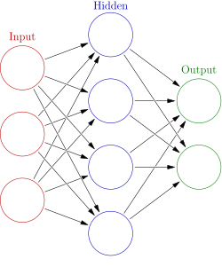
11. Neural Network
Neural Network in simple terms is an interconnected group of nodes which take input along with information from other nodes, develop output without programmed rules.
Build a Neural Network Model from Scratch
model = tf.keras.models.Sequential([
    # The input shape here is the desired size of the image 300x300 ( 3 bytes color )
    # This is the first convolution
    tf.keras.layers.Conv2D(16, (3,3), activation='relu', input_shape=(300, 300, 3)),
    tf.keras.layers.MaxPooling2D(2, 2),

    # The second convolution
    tf.keras.layers.Conv2D(32,(3,3),activation = 'relu'),
    tf.keras.layers.MaxPooling2D(2,2),

    # The third convolution
     tf.keras.layers.Conv2D(64,(3,3),activation = 'relu'),
     tf.keras.layers.MaxPooling2D(2,2),

    # The fourth convolution
     tf.keras.layers.Conv2D(64,(3,3),activation = 'relu'),
     tf.keras.layers.MaxPooling2D(2,2),

    # The fifth convolution
     tf.keras.layers.Conv2D(64,(3,3),activation = 'relu'),
     tf.keras.layers.MaxPooling2D(2,2),

    # The sixth convolution
     tf.keras.layers.Conv2D(64,(3,3),activation = 'relu'),
     tf.keras.layers.MaxPooling2D(2,2),


    # Flatten the results to feed into a DNN
    tf.keras.layers.Flatten(),

    # 512 neuron hidden layer
    tf.keras.layers.Dense(512, activation='relu'),

    # We have only 1 output neuron
    # and it will contain a value from 0-1 where 0 for 1 class ('horses') and 1 for the other ('humans')
    tf.keras.layers.Dense(1, activation='sigmoid')
])
model.summary()
model.compile(loss='binary_crossentropy',
              optimizer=RMSprop(lr=0.001),
              metrics=['accuracy'])
Output —
Model: "sequential"
_________________________________________________________________
Layer (type) Output Shape Param #
=================================================================
conv2d (Conv2D) (None, 298, 298, 16) 448
_________________________________________________________________
max_pooling2d (MaxPooling2D) (None, 149, 149, 16) 0
_________________________________________________________________
conv2d_1 (Conv2D) (None, 147, 147, 32) 4640
_________________________________________________________________
max_pooling2d_1 (MaxPooling2 (None, 73, 73, 32) 0
_________________________________________________________________
conv2d_2 (Conv2D) (None, 71, 71, 64) 18496
_________________________________________________________________
max_pooling2d_2 (MaxPooling2 (None, 35, 35, 64) 0
_________________________________________________________________
conv2d_3 (Conv2D) (None, 33, 33, 64) 36928
_________________________________________________________________
max_pooling2d_3 (MaxPooling2 (None, 16, 16, 64) 0
_________________________________________________________________
conv2d_4 (Conv2D) (None, 14, 14, 64) 36928
_________________________________________________________________
max_pooling2d_4 (MaxPooling2 (None, 7, 7, 64) 0
_________________________________________________________________
conv2d_5 (Conv2D) (None, 5, 5, 64) 36928
_________________________________________________________________
max_pooling2d_5 (MaxPooling2 (None, 2, 2, 64) 0
_________________________________________________________________
flatten (Flatten) (None, 256) 0
_________________________________________________________________
dense (Dense) (None, 512) 131584
_________________________________________________________________
dense_1 (Dense) (None, 1) 513
=================================================================
Total params: 266,465
Trainable params: 266,465
Non-trainable params: 0
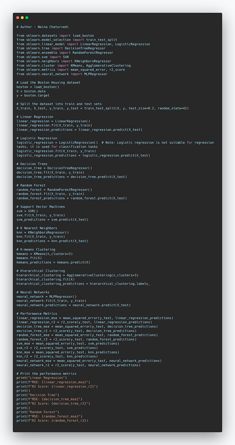
_________________________________________________________________Project Code —
from sklearn.datasets import load_boston
from sklearn.model_selection import train_test_split
from sklearn.linear_model import LinearRegression, LogisticRegression
from sklearn.tree import DecisionTreeRegressor
from sklearn.ensemble import RandomForestRegressor
from sklearn.svm import SVR
from sklearn.neighbors import KNeighborsRegressor
from sklearn.cluster import KMeans, AgglomerativeClustering
from sklearn.metrics import mean_squared_error, r2_score
from sklearn.neural_network import MLPRegressor

# Load the Boston Housing dataset
boston = load_boston()
X = boston.data
y = boston.target

# Split the dataset into train and test sets
X_train, X_test, y_train, y_test = train_test_split(X, y, test_size=0.2, random_state=42)

# Linear Regression
linear_regression = LinearRegression()
linear_regression.fit(X_train, y_train)
linear_regression_predictions = linear_regression.predict(X_test)

# Logistic Regression
logistic_regression = LogisticRegression()  # Note: Logistic regression is not suitable for regression tasks, it is used for classification tasks
logistic_regression.fit(X_train, y_train)
logistic_regression_predictions = logistic_regression.predict(X_test)

# Decision Trees
decision_tree = DecisionTreeRegressor()
decision_tree.fit(X_train, y_train)
decision_tree_predictions = decision_tree.predict(X_test)

# Random Forest
random_forest = RandomForestRegressor()
random_forest.fit(X_train, y_train)
random_forest_predictions = random_forest.predict(X_test)

# Support Vector Machines
svm = SVR()
svm.fit(X_train, y_train)
svm_predictions = svm.predict(X_test)

# K Nearest Neighbors
knn = KNeighborsRegressor()
knn.fit(X_train, y_train)
knn_predictions = knn.predict(X_test)

# K-means Clustering
kmeans = KMeans(n_clusters=3)
kmeans.fit(X)
kmeans_predictions = kmeans.predict(X)

# Hierarchical Clustering
hierarchical_clustering = AgglomerativeClustering(n_clusters=3)
hierarchical_clustering.fit(X)
hierarchical_clustering_predictions = hierarchical_clustering.labels_

# Neural Networks
neural_network = MLPRegressor()
neural_network.fit(X_train, y_train)
neural_network_predictions = neural_network.predict(X_test)

# Performance Metrics
linear_regression_mse = mean_squared_error(y_test, linear_regression_predictions)
linear_regression_r2 = r2_score(y_test, linear_regression_predictions)
decision_tree_mse = mean_squared_error(y_test, decision_tree_predictions)
decision_tree_r2 = r2_score(y_test, decision_tree_predictions)
random_forest_mse = mean_squared_error(y_test, random_forest_predictions)
random_forest_r2 = r2_score(y_test, random_forest_predictions)
svm_mse = mean_squared_error(y_test, svm_predictions)
svm_r2 = r2_score(y_test, svm_predictions)
knn_mse = mean_squared_error(y_test, knn_predictions)
knn_r2 = r2_score(y_test, knn_predictions)
neural_network_mse = mean_squared_error(y_test, neural_network_predictions)
neural_network_r2 = r2_score(y_test, neural_network_predictions)

# Print the performance metrics
print("Linear Regression")
print(f"MSE: {linear_regression_mse}")
print(f"R2 Score: {linear_regression_r2}")
print()
print("Decision Tree")
print(f"MSE: {decision_tree_mse}")
print(f"R2 Score: {decision_tree_r2}")
print()
print("Random Forest")
print(f"MSE: {random_forest_mse}")
print(f"R2 Score: {random_forest_r2})
Snippet —
A project video covering all the Machine Learning Algorithms coming soon ( subscribe today) —
That’s it for 30 days of Data Engineering Series.
Data Engineering projects …coming soon!
Start here Day 1 of Data Engineering :
Let me know if you have questions in the comment section below. Subscribe/ Follow, Like/Clap as it would encourage me to write more in my free time
Stay Tuned!!
Read more —
All the Complete System Design Series Parts —
6. Networking, How Browsers work, Content Network Delivery ( CDN)
Github —
For Python Projects —
For complete 60 days of Data Science and ML : Day 1 — Day 60 : Quick Recap of 60 days of Data Science and ML
Follow for more updates. Stay tuned and keep coding!
For other projects, tune to —
Build Machine Learning Pipelines( With Code)
Recurrent Neural Network with Keras
Clustering Geolocation Data in Python using DBSCAN and K-Means
Facial Expression Recognition using Keras
Hyperparameter Tuning with Keras Tuner
Custom Layers in Keras


