
Day 28 of 30 days of Data Analytics with Projects Series — Regression( Part 1)
Welcome back peep. Hope all’s well. This is Day 28 of 30 days of data analytics where we will be covering Regression ( Part 1).
1.Linear Regression
2. Multi Linear Regression
3. Polynomial Regression
Part 2
4. Support Vector Regression
5. Decision Tree Regression
6. Random Forest Regression
Let’s cover the most important concepts in brief —
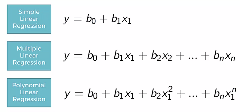
- Linear Regression: a statistical method used to analyze the relationship between one dependent variable and one or more independent variables by fitting a linear equation to the observed data.
- Multi Linear Regression: a statistical method used to analyze the relationship between one dependent variable and two or more independent variables by fitting a linear equation to the observed data.
- Polynomial Regression: a form of regression analysis in which the relationship between the independent variable x and the dependent variable y is modeled as an nth degree polynomial.
- Support Vector Regression: a type of support vector machine that is used for regression problems. It uses the same basic idea as SVM for classification, but the algorithm is adapted for regression.
- Decision Tree Regression: a type of decision tree used for regression problems. It creates a model that predicts a value for a given input.
- Random Forest Regression: a type of ensemble learning method for regression problems, where a number of decision trees are created and combined to make a final prediction.
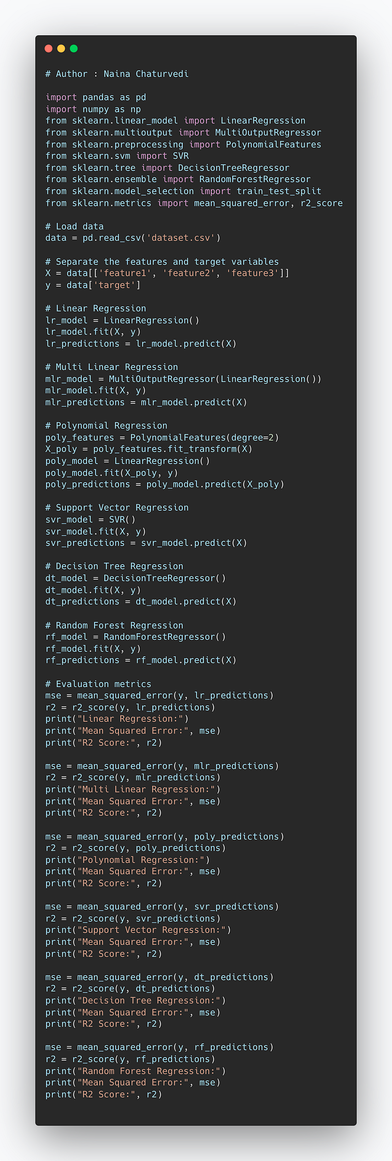
Complete Code Implementation —
import pandas as pd
import numpy as np
from sklearn.linear_model import LinearRegression
from sklearn.multioutput import MultiOutputRegressor
from sklearn.preprocessing import PolynomialFeatures
from sklearn.svm import SVR
from sklearn.tree import DecisionTreeRegressor
from sklearn.ensemble import RandomForestRegressor
from sklearn.model_selection import train_test_split
from sklearn.metrics import mean_squared_error, r2_score

# Load data
data = pd.read_csv('dataset.csv')

# Separate the features and target variables
X = data[['feature1', 'feature2', 'feature3']]
y = data['target']

# Linear Regression
lr_model = LinearRegression()
lr_model.fit(X, y)
lr_predictions = lr_model.predict(X)

# Multi Linear Regression
mlr_model = MultiOutputRegressor(LinearRegression())
mlr_model.fit(X, y)
mlr_predictions = mlr_model.predict(X)

# Polynomial Regression
poly_features = PolynomialFeatures(degree=2)
X_poly = poly_features.fit_transform(X)
poly_model = LinearRegression()
poly_model.fit(X_poly, y)
poly_predictions = poly_model.predict(X_poly)

# Support Vector Regression
svr_model = SVR()
svr_model.fit(X, y)
svr_predictions = svr_model.predict(X)

# Decision Tree Regression
dt_model = DecisionTreeRegressor()
dt_model.fit(X, y)
dt_predictions = dt_model.predict(X)

# Random Forest Regression
rf_model = RandomForestRegressor()
rf_model.fit(X, y)
rf_predictions = rf_model.predict(X)

# Evaluation metrics
mse = mean_squared_error(y, lr_predictions)
r2 = r2_score(y, lr_predictions)
print("Linear Regression:")
print("Mean Squared Error:", mse)
print("R2 Score:", r2)

mse = mean_squared_error(y, mlr_predictions)
r2 = r2_score(y, mlr_predictions)
print("Multi Linear Regression:")
print("Mean Squared Error:", mse)
print("R2 Score:", r2)

mse = mean_squared_error(y, poly_predictions)
r2 = r2_score(y, poly_predictions)
print("Polynomial Regression:")
print("Mean Squared Error:", mse)
print("R2 Score:", r2)

mse = mean_squared_error(y, svr_predictions)
r2 = r2_score(y, svr_predictions)
print("Support Vector Regression:")
print("Mean Squared Error:", mse)
print("R2 Score:", r2)

mse = mean_squared_error(y, dt_predictions)
r2 = r2_score(y, dt_predictions)
print("Decision Tree Regression:")
print("Mean Squared Error:", mse)
print("R2 Score:", r2)

mse = mean_squared_error(y, rf_predictions)
r2 = r2_score(y, rf_predictions)
print("Random Forest Regression:")
print("Mean Squared Error:", mse)
print("R2 Score:", r2)
Snippet —
What’s covered in 30 days of Data Analytics Series till now —
Day 1 : Data Analytics basics and kickstart of Data analytics with projects series
Day 3 : Data Analytics Ecosystem — Data Life Cycle, Data Analysis complete process ( most important things)
Day 5 : Statistics
Day 6 : Basic and Advanced SQL
Day 8 : Pandas and Numpy
Day 9 : Data Manipulation
Day 10 : Data Visualization — Part 1
Day 11 : Project 1 : Data Visualization — Part 2
Day 12 : Data Visualization — Part 3
Day 13: Tableau — Part 1
Day 14: Tableau — Part 2
Day 15: Tableau — Part 3
Day 16 : Data Analysis Project 2
Day 17 : Data Analysis Project 3
Day 18: Data Analysis Project 4
Day 20 : Data Analysis Project 6
Day 21 : Data Analysis Project 7
Take Complete Hands On Tableau Course : Link
Projects Videos —
All the projects, data structures, SQL, algorithms, system design, Data Science and ML , Data Analytics, Data Engineering, , Implemented Data Science and ML projects, Implemented Data Engineering Projects, Implemented Deep Learning Projects, Implemented Machine Learning Ops Projects, Implemented Time Series Analysis and Forecasting Projects, Implemented Applied Machine Learning Projects, Implemented Tensorflow and Keras Projects, Implemented PyTorch Projects, Implemented Scikit Learn Projects, Implemented Big Data Projects, Implemented Cloud Machine Learning Projects, Implemented Neural Networks Projects, Implemented OpenCV Projects,Complete ML Research Papers Summarized, Implemented Data Analytics projects, Implemented Data Visualization Projects, Implemented Data Mining Projects, Implemented Natural Leaning Processing Projects, MLOps and Deep Learning, Applied Machine Learning with Projects Series, PyTorch with Projects Series, Tensorflow and Keras with Projects Series, Scikit Learn Series with Projects, Time Series Analysis and Forecasting with Projects Series, ML System Design Case Studies Series videos will be published on our youtube channel ( just launched).
Subscribe today!
Tech Newsletter —
If you are interested, you can join my newsletter through which I send tech interview tips, techniques, patterns, hacks — Software Development, ML, Data Science, Startups and Technology projects to more than 30K readers. You can subscribe to Tech Brew :
Let’s get started!
Simple Linear Regression
It’s a technique to estimate the relationship between two quantitative variables. It is used when you want to establish:
- Strength of the relationship — How strong the relationship is between two variables
- The value of the dependent variable at a certain value of the independent variable.
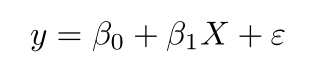
where,
y is the predicted value of the dependent variable for any given value of the independent variable which is X.
B0 is the intercept and B1 is the regression coefficient
x is the independent variable
e is the error of the estimate
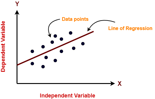
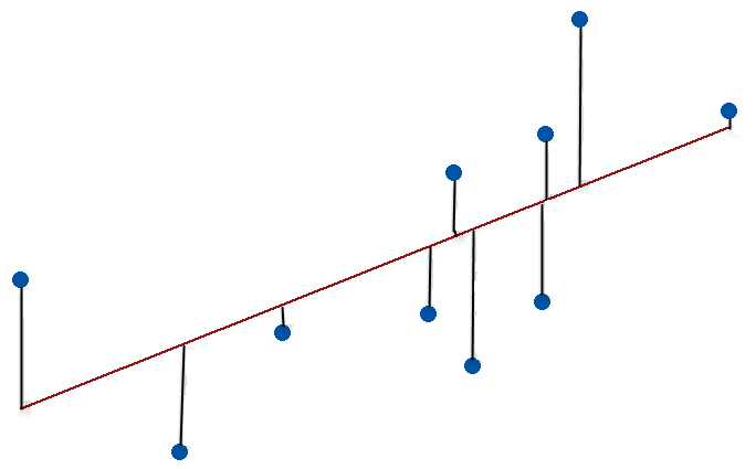
It works on the assumption that the relationship between the independent and dependent variable is linear: the line of best fit through the data points is a straight line as shown in the diagram.
from sklearn.linear_model import LinearRegression
regressor = LinearRegression()
regressor.fit(I_Train_data, D_Train_data)
preds = regressor.predict(X_test)
Visualize the training and test set
Training set results —
import matplotlib.pyplot as plt# Visualizing the Training set results
plt.scatter(X_train, y_train, color = 'green')
plt.plot(X_train, regressor.predict(X_train), color = 'blue')
plt.xlabel('Independent Variable set')
plt.ylabel('Dependent Variable set')
plt.show()Test set results —
# Visualizing the Test set results
plt.scatter(X_test, y_test, color = 'green')
plt.plot(X_train, regressor.predict(X_train), color = 'blue')
plt.xlabel('Independent Variable set')
plt.ylabel('Dependent Variable set')
plt.show()
Linear regression uses mean-square error (MSE) to calculate the error of the model. MSE is calculated by:
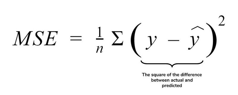
Measure the distance of the observed y-values from the predicted y-values at each value of x;
Square each of these distances and calculate the mean of each of the squared distances.
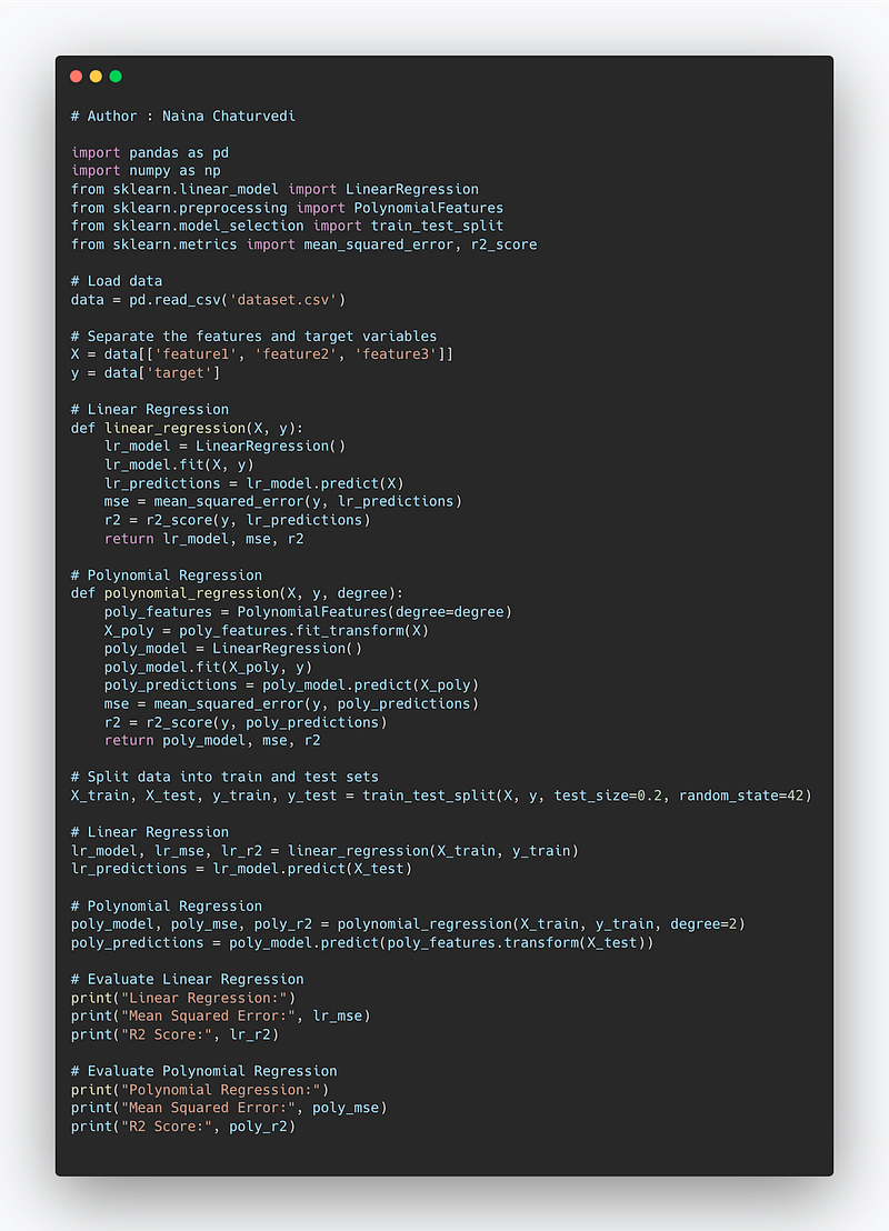
Code Implementation —
import pandas as pd
import numpy as np
from sklearn.linear_model import LinearRegression
from sklearn.preprocessing import PolynomialFeatures
from sklearn.model_selection import train_test_split
from sklearn.metrics import mean_squared_error, r2_score

# Load data
data = pd.read_csv('dataset.csv')

# Separate the features and target variables
X = data[['feature1', 'feature2', 'feature3']]
y = data['target']

# Linear Regression
def linear_regression(X, y):
    lr_model = LinearRegression()
    lr_model.fit(X, y)
    lr_predictions = lr_model.predict(X)
    mse = mean_squared_error(y, lr_predictions)
    r2 = r2_score(y, lr_predictions)
    return lr_model, mse, r2

# Polynomial Regression
def polynomial_regression(X, y, degree):
    poly_features = PolynomialFeatures(degree=degree)
    X_poly = poly_features.fit_transform(X)
    poly_model = LinearRegression()
    poly_model.fit(X_poly, y)
    poly_predictions = poly_model.predict(X_poly)
    mse = mean_squared_error(y, poly_predictions)
    r2 = r2_score(y, poly_predictions)
    return poly_model, mse, r2

# Split data into train and test sets
X_train, X_test, y_train, y_test = train_test_split(X, y, test_size=0.2, random_state=42)

# Linear Regression
lr_model, lr_mse, lr_r2 = linear_regression(X_train, y_train)
lr_predictions = lr_model.predict(X_test)

# Polynomial Regression
poly_model, poly_mse, poly_r2 = polynomial_regression(X_train, y_train, degree=2)
poly_predictions = poly_model.predict(poly_features.transform(X_test))

# Evaluate Linear Regression
print("Linear Regression:")
print("Mean Squared Error:", lr_mse)
print("R2 Score:", lr_r2)

# Evaluate Polynomial Regression
print("Polynomial Regression:")
print("Mean Squared Error:", poly_mse)
print("R2 Score:", poly_r2)
Snippet —
Multi Linear Regression
It’s used to estimate the relationship between two or more independent variables and one dependent variable. It is used when you want to establish:
- Strength of the relationship — How strong the relationship is between two or more independent variables and one dependent variable
- The value of the dependent variable at a certain value of the independent variable.
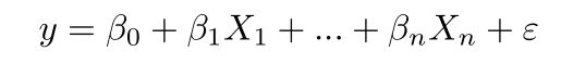
B0 = the y-intercept
B1X1= the regression coefficient (b1) of the first independent variable (x1)
BnXn = the regression coefficient of the last independent variable
y = the predicted value of the dependent variable
e = model error
Assumptions of Linear Regression
Linearity
Independence of errors
Homoscedasticity
Multivariate normality
Lack of multi collinearity
In order to find best fit line, it calculates 3 parameters —
- The t-stat of the model
- The associated p-value
- Regression coefficients
# Fitting multiple lineaar regression to the training set
from sklearn.linear_model import LinearRegression
regressor = LinearRegression()
regressor.fit(X_train, y_train)
# Predicting the test set results
y_pred = regressor.predict(X_test)X = np.append(arr = np.ones((20, 1)).astype(int), values = X, axis = 1)
X_opt = X[:, [0, 1, 2, 3, 4, 5]]
regressor_OLS = sm.OLS(endog = y, exog = X_opt).fit()
regressor_OLS.summary()
X_opt = X[:, [0, 1, 3, 4, 5]]
regressor_OLS = sm.OLS(endog=y, exog=X_opt).fit()
regressor_OLS.summary()
X_opt = X[:, [0, 3, 4, 5]]
regressor_OLS = sm.OLS(endog=y, exog=X_opt).fit()
regressor_OLS.summary()
X_opt = X[:, [0, 3, 5]]
regressor_OLS = sm.OLS(endog=y, exog=X_opt).fit()
regressor_OLS.summary()
X_opt = X[:, [0, 3]]
regressor_OLS = sm.OLS(endog=y, exog=X_opt).fit()
regressor_OLS.summary()Polynomial Regression
In polynomial Regression, the relationship between the independent variable x and dependent variable y is established as the nth degree polynomial providing the best approximation of the relationship between dependent and independent variables.
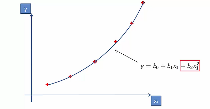
It fits a nonlinear relationship between the value of x and conditional mean of y. For cases where data points are arranged in a non-linear fashion, we need the Polynomial Regression model.
# Fitting Polynomial Regression to the datasetfrom sklearn.preprocessing import PolynomialFeaturespoly = PolynomialFeatures(degree = 3) X_poly = poly.fit_transform(X) poly.fit(X_poly, y) l = LinearRegression() l.fit(X_poly, y)
Visualize —
plt.scatter(X, y, color = 'green')
plt.plot(X, l.predict(poly.fit_transform(X)), color = 'red')
plt.title('Polynomial Regression')
plt.show()
Complete Code Implementation —
import numpy as np
import matplotlib.pyplot as plt
from sklearn.linear_model import LinearRegression
from sklearn.linear_model import MultiTaskLasso, Lasso
from sklearn.preprocessing import PolynomialFeatures
from sklearn.svm import SVR
from sklearn.tree import DecisionTreeRegressor
from sklearn.ensemble import RandomForestRegressor

# Generate sample data for regression
X = np.random.rand(100, 1) * 10
y = 2 * X + np.random.randn(100, 1)

# Linear Regression
linear_model = LinearRegression()
linear_model.fit(X, y)
linear_predictions = linear_model.predict(X)

# Multi-Linear Regression
multi_linear_model = MultiTaskLasso(alpha=0.1)
multi_linear_model.fit(X, y)
multi_linear_predictions = multi_linear_model.predict(X)

# Polynomial Regression
polynomial_features = PolynomialFeatures(degree=2)
X_poly = polynomial_features.fit_transform(X)
polynomial_model = LinearRegression()
polynomial_model.fit(X_poly, y)
polynomial_predictions = polynomial_model.predict(X_poly)

# Support Vector Regression
svr_model = SVR(kernel='linear')
svr_model.fit(X, y.flatten())
svr_predictions = svr_model.predict(X)

# Decision Tree Regression
dt_model = DecisionTreeRegressor()
dt_model.fit(X, y)
dt_predictions = dt_model.predict(X)

# Random Forest Regression
rf_model = RandomForestRegressor(n_estimators=100)
rf_model.fit(X, y.flatten())
rf_predictions = rf_model.predict(X)

# Plotting the results
plt.scatter(X, y, color='blue', label='Actual Data')
plt.plot(X, linear_predictions, color='red', label='Linear Regression')
plt.plot(X, multi_linear_predictions, color='green', label='Multi-Linear Regression')
plt.plot(X, polynomial_predictions, color='orange', label='Polynomial Regression')
plt.plot(X, svr_predictions, color='purple', label='Support Vector Regression')
plt.plot(X, dt_predictions, color='brown', label='Decision Tree Regression')
plt.plot(X, rf_predictions, color='magenta', label='Random Forest Regression')
plt.xlabel('X')
plt.ylabel('y')
plt.title('Regression Models')
plt.legend()
plt.show()- Linear Regression: We use the
LinearRegressionclass from scikit-learn to fit a linear equation to the data and predict the values. - Multi-Linear Regression: We use the
MultiTaskLassoclass from scikit-learn to fit a linear equation with multiple targets (in this case, only one target) and predict the values. - Polynomial Regression: We use the
PolynomialFeaturesclass to transform the original features into polynomial features, and then fit a linear equation usingLinearRegressionto predict the values. - Support Vector Regression: We use the
SVRclass from scikit-learn to perform Support Vector Regression with a linear kernel and predict the values. - Decision Tree Regression: We use the
DecisionTreeRegressorclass from scikit-learn to fit a decision tree model and predict the values. - Random Forest Regression: We use the
RandomForestRegressorclass from scikit-learn to fit an ensemble of decision trees and predict the values.
That’s it for now.
Find Day 29 Below : Decision Tree Regression, Support Vector Regression and Random Forest Regression.
Let me know if you have questions in the comment section below. Subscribe/ Follow, Like/Clap as it would encourage me to write more in my free time
Stay Tuned!!
Read More —
11 most important System Design Base Concepts
6. Networking, How Browsers work, Content Network Delivery ( CDN)
13. System Design Template — How to solve any System Design Question
System Design Case Studies — In Depth
Complete Data Structures and Algorithm Series
Some of the other best Series —
30 days of Data Structures and Algorithms and System Design Simplified
Data Science and Machine Learning Research ( papers) Simplified **
100 days : Your Data Science and Machine Learning Degree Series with projects
Complete Data Visualization and Pre-processing Series with projects
Exceptional Github Repos — Part 1
Exceptional Github Repos — Part 2
Tech Newsletter —
If you are interested, you can join my newsletter through which I send tech interview tips, techniques, patterns, hacks — Software Development, ML, Data Science, Startups and Technology projects to more than 30K readers. You can subscribe to Tech Brew :
For Python Projects —
For complete 60 days of Data Science and ML : Day 1 — Day 60 : Quick Recap of 60 days of Data Science and ML
Follow for more updates. Stay tuned and keep coding!
For other projects, tune to —
Build Machine Learning Pipelines( With Code)
Recurrent Neural Network with Keras
Clustering Geolocation Data in Python using DBSCAN and K-Means
Facial Expression Recognition using Keras
Hyperparameter Tuning with Keras Tuner
Custom Layers in Keras


