
Day 4 of 30 days of Data Analytics with Projects Series
Welcome back peeps. Happy to share that we have just finished —
Finished Series —
60 Days of Data Science and Machine Learning with projects Series
We are now starting a new series — 30 days of Data Analytics with Projects. This series would run in parallel with —
Ongoing Series —
What’s covered till now —
Day 1 : Data Analytics basics and kickstart of Data analytics with projects series
Day 3 : Data Analytics Ecosystem — Data Life Cycle, Data Analysis complete process ( most important things)
Day 5 : Statistics
Projects Videos —
All the projects, data structures, SQL, algorithms, system design, Data Science and ML , Data Analytics, Data Engineering, , Implemented Data Science and ML projects, Implemented Data Engineering Projects, Implemented Deep Learning Projects, Implemented Machine Learning Ops Projects, Implemented Time Series Analysis and Forecasting Projects, Implemented Applied Machine Learning Projects, Implemented Tensorflow and Keras Projects, Implemented PyTorch Projects, Implemented Scikit Learn Projects, Implemented Big Data Projects, Implemented Cloud Machine Learning Projects, Implemented Neural Networks Projects, Implemented OpenCV Projects,Complete ML Research Papers Summarized, Implemented Data Analytics projects, Implemented Data Visualization Projects, Implemented Data Mining Projects, Implemented Natural Leaning Processing Projects, MLOps and Deep Learning, Applied Machine Learning with Projects Series, PyTorch with Projects Series, Tensorflow and Keras with Projects Series, Scikit Learn Series with Projects, Time Series Analysis and Forecasting with Projects Series, ML System Design Case Studies Series videos will be published on our youtube channel ( just launched).
Subscribe today!
For Day 4 we will cover Probability. Let’s dive in!
Probability is a measure of the likelihood of an event occurring. It is typically expressed as a decimal or a percentage between 0 and 1, with 0 indicating that an event is impossible and 1 indicating that an event is certain.
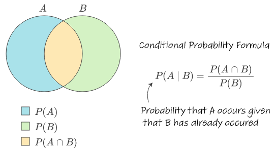
- Conditional probability is the probability of an event occurring given that another event has already occurred. It is represented as P(A|B), which is the probability of event A occurring given that event B has already occurred.
# Example code for conditional probability

# Calculate the conditional probability P(A|B)
def calculate_conditional_probability(A, B):
    # Calculate the joint probability P(A and B)
    joint_probability = P_A_and_B(A, B)

    # Calculate the probability P(B)
    probability_B = P(B)

    # Calculate the conditional probability P(A|B)
    conditional_probability = joint_probability / probability_B

    return conditional_probability

# Example usage
event_A = "Event A"
event_B = "Event B"

# Calculate P(A|B)
conditional_probability = calculate_conditional_probability(event_A, event_B)
print(f"The conditional probability of {event_A} given {event_B} is: {conditional_probability}")- Binomial Distribution is a probability distribution that describes the number of success in a fixed number of independent trials. It is used to model the number of successes in a fixed number of trials when the probability of success is constant.
# Example code for binomial distribution

from scipy.stats import binom

# Define the parameters of the binomial distribution
n = 10  # Number of trials
p = 0.5  # Probability of success

# Create a binomial distribution object
binomial_dist = binom(n, p)

# Calculate the probability mass function (PMF) for k successes
k = 3
probability = binomial_dist.pmf(k)

print(f"The probability of {k} successes in {n} trials with a success probability of {p} is: {probability}")- Probability Density Function (PDF) is a function that describes the probability distribution of a continuous random variable. It gives the probability that a random variable will take on a certain value, rather than falling within a certain range of values.
# Example code for probability density function (PDF)

from scipy.stats import norm

# Define the parameters of the normal distribution
mu = 0  # Mean
sigma = 1  # Standard deviation

# Create a normal distribution object
normal_dist = norm(mu, sigma)

# Calculate the probability density function (PDF) for x
x = 1.5
pdf_value = normal_dist.pdf(x)

print(f"The probability density function (PDF) at x = {x} is: {pdf_value}")- Sampling Distribution is the distribution of the sample mean or other statistics, when the samples are selected randomly from a population. It is used to understand the behavior of a statistic when the samples are randomly selected from a population.
# Example code for sampling distribution

import numpy as np

# Generate random samples from a population
population = np.random.normal(0, 1, 1000)

# Select a sample from the population
sample_size = 100
sample = np.random.choice(population, size=sample_size, replace=False)

# Calculate the sample mean
sample_mean = np.mean(sample)

print(f"The sample mean is: {sample_mean}")
In summary, probability is a measure of the likelihood of an event occurring, conditional probability is the probability of an event given that another event has already occurred, Binomial Distribution is a probability distribution that describes the number of success in a fixed number of independent trials, PDF is a function that describes the probability distribution of a continuous random variable, and Sampling Distribution is the distribution of the sample mean or other statistics when the samples are selected randomly from a population.
Probability
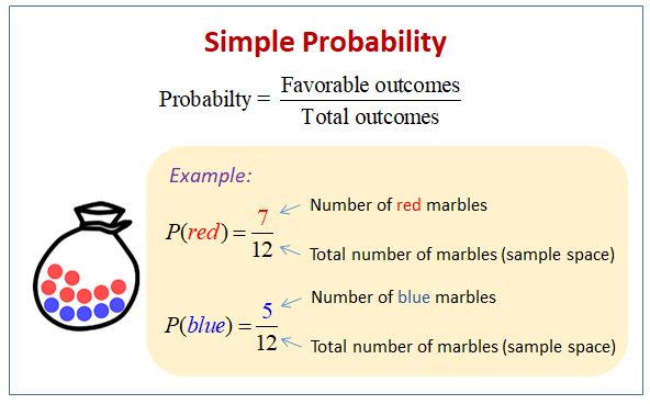
In layman terms, probability defines the likelihood of an event’s occurrence. It’s defined as the ratio of the no of favorable outcomes to the total no of outcomes of an event.
Probability of event to happen P(E) = Number of favourable outcomes/Total Number of outcomes
Some terms that are important to know in probability space -
- Sample space : It means all the possible outcomes of an experiment
- Trial : It means a random experiment
- Population: It’s an identified group of individuals
- Variable: It’s a measurable factor or condition that exists in different amounts or types
- Effect Size: Conveys how much difference there is between averages of variables
- Exhaustive events : It means when the set of the outcomes is equal to the sample space.
- Mutual exhaustive events :It means the events that cannot happen at the same time.
- Random Sampling: It’s a (random) way of selecting individuals from a population that makes sure that every individual has an equal probability of being selected
- Point Estimate: It’s an estimate of some value in a population, such as an average
- Confidence Intervals: It’s the range of values around point estimates that likely contain the true value of a variable in the population/sample
- Margin of Error: Used for estimating miscalculation or errors, It’s a calculated amount added and subtracted to a point estimate
- Standard Deviation: The average distance between each data point and the total average
Code implementation —
Trial
# Example code for trial

import random

# Define a trial function for flipping a coin
def coin_trial():
    outcomes = ['Heads', 'Tails']
    return random.choice(outcomes)

# Perform a coin trial
result = coin_trial()

print("Trial Result:")
print(result)
Effect Size
# Example code for effect size

# Calculate the effect size (difference in means)
mean1 = 8
mean2 = 6
effect_size = mean1 - mean2

print("Effect Size:")
print(effect_size)
Random Sampling
# Example code for random sampling

import random

# Define a population
population = [1, 2, 3, 4, 5, 6, 7, 8, 9, 10]

# Perform random sampling
sample_size = 5
sample = random.sample(population, sample_size)

print("Random Sample:")
print(sample)
Point Estimate
# Example code for point estimate

import numpy as np

# Define a sample
sample = [15, 20, 25, 18, 22]

# Calculate the point estimate (sample mean)
point_estimate = np.mean(sample)

print("Point Estimate:")
print(point_estimate)
Confidence Intervals
# Example code for confidence intervals

import numpy as np
from scipy.stats import t

# Define a sample
sample = [15, 20, 25, 18, 22]

# Calculate the confidence interval
confidence_level = 0.95
sample_mean = np.mean(sample)
sample_std = np.std(sample, ddof=1)
sample_size = len(sample)
margin_of_error = t.ppf((1 + confidence_level) / 2, sample_size - 1) * sample_std / np.sqrt(sample_size)
confidence_interval = (sample_mean - margin_of_error, sample_mean + margin_of_error)

print("Confidence Interval:")
print(confidence_interval)
Margin of Error
# Example code for margin of error

import numpy as np
from scipy.stats import t

# Define a sample
sample = [15, 20, 25, 18, 22]

# Calculate the margin of error
confidence_level = 0.95
sample_std = np.std(sample, ddof=1)
sample_size = len(sample)
margin_of_error = t.ppf((1 + confidence_level) / 2, sample_size - 1) * sample_std / np.sqrt(sample_size)

print("Margin of Error:")
print(margin_of_error)
Standard Deviation
# Example code for standard deviation

import numpy as np

# Define a dataset
data = [2, 4, 6, 8, 10]

# Calculate the standard deviation
std_dev = np.std(data)

print("Standard Deviation:")
print(std_dev)
Conditional Probability
Conditional Probability defined the likelihood of an event based on the occurrence of a previous event.
# Example code for conditional probability

# Calculate the conditional probability P(A|B)
def calculate_conditional_probability(A, B):
    # Calculate the joint probability P(A and B)
    joint_probability = P_A_and_B(A, B)

    # Calculate the probability P(B)
    probability_B = P(B)

    # Calculate the conditional probability P(A|B)
    conditional_probability = joint_probability / probability_B

    return conditional_probability

# Example usage
event_A = "Event A"
event_B = "Event B"

# Calculate P(A|B)
conditional_probability = calculate_conditional_probability(event_A, event_B)
print(f"The conditional probability of {event_A} given {event_B} is: {conditional_probability}")
Binomial Distribution
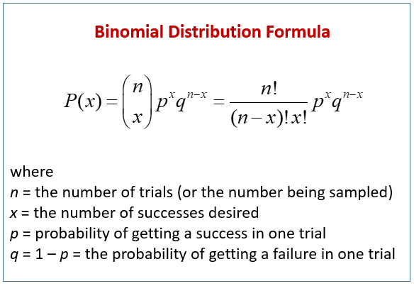
Binomial distribution defines the likelihood of getting a certain outcomes when doing a series of tests for which there are only two possible outcomes.
# Example code for binomial distribution

from scipy.stats import binom

# Define the parameters of the binomial distribution
n = 10  # Number of trials
p = 0.5  # Probability of success

# Create a binomial distribution object
binomial_dist = binom(n, p)

# Calculate the probability mass function (PMF) for k successes
k = 3
probability = binomial_dist.pmf(k)

print(f"The probability of {k} successes in {n} trials with a success probability of {p} is: {probability}")
Sampling Distribution
Sampling distribution defines a probability distribution of a measure/statistic that’s obtained from a large no of samples which are drawn from a specific set of population.
To summarize, the probability distribution of a statistic is called sampling distribution.
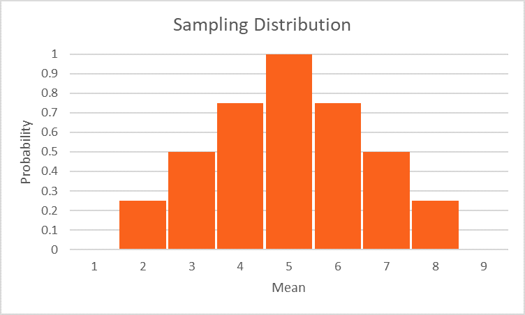
It helps calculate a frequency distribution of each sample statistic.
# Example code for sampling distribution

import numpy as np

# Generate random samples from a population
population = np.random.normal(0, 1, 1000)

# Select a sample from the population
sample_size = 100
sample = np.random.choice(population, size=sample_size, replace=False)

# Calculate the sample mean
sample_mean = np.mean(sample)

print(f"The sample mean is: {sample_mean}")
Normal Distribution —
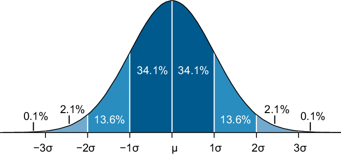
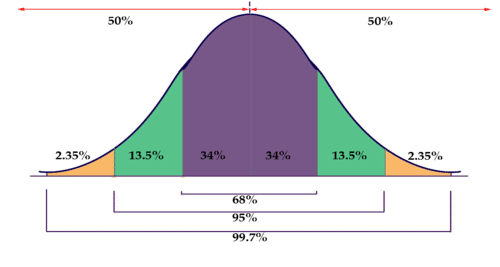
Also known as continuous random variable, the variable can take any value.
Implementation —
from scipy.stats import norm
import numpy as np
arr2 = np.array([0.91,0.17,0.99996833, 0.81, 0.97,0.54])
print(norm.ppf(arr2))
Output —
[ 1.34075503 -0.95416525 4.00000928 0.8778963 1.88079361 0.10043372]Probability Density Function
Probability Density Function defines the likelihood of an outcomes for discrete/continuous random variables.
# Example code for probability density function (PDF)

from scipy.stats import norm

# Define the parameters of the normal distribution
mu = 0  # Mean
sigma = 1  # Standard deviation

# Create a normal distribution object
normal_dist = norm(mu, sigma)

# Calculate the probability density function (PDF) for x
x = 1.5
pdf_value = normal_dist.pdf(x)

print(f"The probability density function (PDF) at x = {x} is: {pdf_value}")
Bayes Theorem
Bayes’ Theorem is a fundamental concept in probability that allows us to update the probability of an event based on new evidence. It is expressed as P(A|B) = (P(B|A) * P(A)) / P(B).
# Example code for Bayes' Theorem

# Calculate the posterior probability using Bayes' Theorem
def calculate_posterior_probability(P_A, P_B_given_A, P_B):
    posterior_probability = (P_B_given_A * P_A) / P_B
    return posterior_probability

# Example usage
P_A = 0.3  # Prior probability of event A
P_B_given_A = 0.7  # Probability of event B given event A
P_B = 0.5  # Probability of event B

# Calculate the posterior probability P(A|B)
posterior_probability = calculate_posterior_probability(P_A, P_B_given_A, P_B)
print(f"The posterior probability of event A given event B is: {posterior_probability}")
Central Limit Theorem
The Central Limit Theorem states that the sampling distribution of the sample mean approaches a normal distribution as the sample size increases, regardless of the shape of the population distribution.
# Example code for Central Limit Theorem

import numpy as np
import matplotlib.pyplot as plt

# Generate random samples from a population
population = np.random.normal(0, 1, 1000)

# Select multiple samples from the population
sample_size = 100
num_samples = 1000

sample_means = []

for _ in range(num_samples):
    sample = np.random.choice(population, size=sample_size, replace=False)
    sample_mean = np.mean(sample)
    sample_means.append(sample_mean)

# Plot the sampling distribution
plt.hist(sample_means, bins=30, density=True, alpha=0.7)
plt.xlabel("Sample Mean")
plt.ylabel("Probability")
plt.title("Sampling Distribution")
plt.show()
Hypothesis Testing
Hypothesis testing is a statistical method used to make inferences or draw conclusions about a population based on sample data. It involves stating a null hypothesis and an alternative hypothesis, calculating test statistics, and comparing it to a critical value or p-value.
# Example code for hypothesis testing

from scipy.stats import ttest_ind

# Define two samples
sample1 = [10, 12, 15, 13, 11]
sample2 = [14, 16, 18, 17, 19]

# Perform a t-test
t_statistic, p_value = ttest_ind(sample1, sample2)

print("T-Statistic:", t_statistic)
print("P-Value:", p_value)
Monte Carlo Simulation
Monte Carlo simulation is a technique that uses random sampling to estimate probabilities and analyze complex systems or processes. It involves generating random numbers based on specified distributions and running simulations to obtain numerical results.
# Example code for Monte Carlo simulation

import random

# Perform Monte Carlo simulation to estimate pi
num_points = 1000000
points_inside_circle = 0

for _ in range(num_points):
    x = random.uniform(-1, 1)
    y = random.uniform(-1, 1)

    if x**2 + y**2 <= 1:
        points_inside_circle += 1

pi_estimate = 4 * points_inside_circle / num_points

print("Estimated Value of Pi:", pi_estimate)
That’s it for now. Day 5 : Coming Soon!
Let me know if you have questions in the comment section below. Subscribe/ Follow, Like/Clap as it would encourage me to write more in my free time
Stay Tuned!!
Read More —
11 most important System Design Base Concepts
6. Networking, How Browsers work, Content Network Delivery ( CDN)
13. System Design Template — How to solve any System Design Question
System Design Case Studies — In Depth
Complete Data Structures and Algorithm Series
Some of the other best Series —
30 days of Data Structures and Algorithms and System Design Simplified
Data Science and Machine Learning Research ( papers) Simplified **
100 days : Your Data Science and Machine Learning Degree Series with projects
Complete Data Visualization and Pre-processing Series with projects
Exceptional Github Repos — Part 1
Exceptional Github Repos — Part 2
Tech Newsletter —
If you are interested, you can join my newsletter through which I send tech interview tips, techniques, patterns, hacks — Software Development, ML, Data Science, Startups and Technology projects to more than 30K readers. You can subscribe to Tech Brew :
For Python Projects —
For complete 60 days of Data Science and ML : Day 1 — Day 60 : Quick Recap of 60 days of Data Science and ML
Follow for more updates. Stay tuned and keep coding!
For other projects, tune to —
Build Machine Learning Pipelines( With Code)
Recurrent Neural Network with Keras
Clustering Geolocation Data in Python using DBSCAN and K-Means
Facial Expression Recognition using Keras
Hyperparameter Tuning with Keras Tuner
Custom Layers in Keras


