Implemented Big Data Projects

Repo for all the projects ( vertical post)…

Welcome back peeps.

Since we are now focusing on our goals for 2023 — new vertical series than horizontal ( means you will find all the contents of the series in one post and projects in second than developing/extending it to new posts every time). So, keep checking this post every day to see new projects.

Prerequisite to these projects —

Complete 60 days of Data Science and Machine Learning before starting this series ( link below) —

Projects Videos —

All the projects, data structures, SQL, algorithms, system design, Data Science and ML , Data Analytics, Data Engineering, , Implemented Data Science and ML projects, Implemented Data Engineering Projects, Implemented Deep Learning Projects, Implemented Machine Learning Ops Projects, Implemented Time Series Analysis and Forecasting Projects, Implemented Applied Machine Learning Projects, Implemented Tensorflow and Keras Projects, Implemented PyTorch Projects, Implemented Scikit Learn Projects, Implemented Big Data Projects, Implemented Cloud Machine Learning Projects, Implemented Neural Networks Projects, Implemented OpenCV Projects,Complete ML Research Papers Summarized, Implemented Data Analytics projects, Implemented Data Visualization Projects, Implemented Data Mining Projects, Implemented Natural Leaning Processing Projects, MLOps and Deep Learning, Applied Machine Learning with Projects Series, PyTorch with Projects Series, Tensorflow and Keras with Projects Series, Scikit Learn Series with Projects, Time Series Analysis and Forecasting with Projects Series, ML System Design Case Studies Series videos will be published on our youtube channel ( just launched).

Subscribe today!

Tech Newsletter —

If you are interested, you can join my newsletter through which I send tech interview tips, techniques, patterns, hacks — Software Development, ML, Data Science, Startups and Technology projects to more than 35K readers. You can subscribe to Ignito:

Let’s dive in!

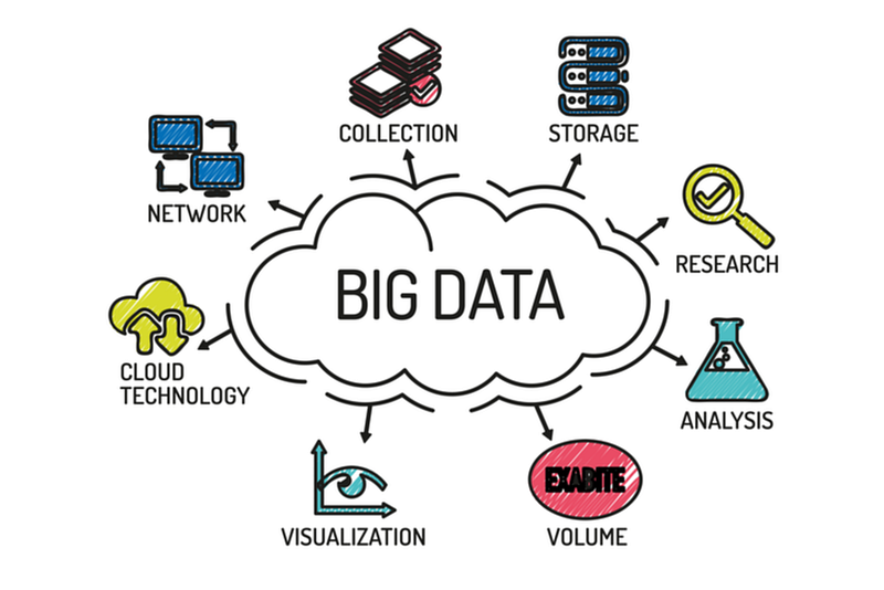
Big data refers to the large and complex sets of data that traditional data processing techniques are unable to handle. It includes structured and unstructured data, such as text, images, videos, and sensor data, as well as data from social media, e-commerce, and IoT devices. The volume, velocity, and variety of big data can make it challenging to process, store, and analyze.

Big data techniques are the methods and tools used to process, store, and analyze big data. Some of the most common big data techniques include:

• Hadoop: A distributed file system and a framework for running large-scale data processing tasks on clusters of commodity hardware.
• MapReduce: A programming model for processing large data sets in parallel across a cluster of computers.
• Spark: An open-source, distributed computing system that can process large data sets quickly.
• NoSQL databases: Non-relational databases that can handle large amounts of unstructured data and handle high write loads.
• Cloud computing: Allows storing and processing large amounts of data using scalable and cost-effective cloud-based services, such as Amazon S3, Google Cloud Storage, and Microsoft Azure Blob Storage.
• Data warehousing and Business Intelligence (BI) tools: Tools for storing, managing, and analyzing large amounts of data, such as Amazon Redshift, Google BigQuery, and Microsoft Azure Synapse Analytics.
• Machine learning and artificial intelligence: Techniques for analyzing and making predictions from large data sets, such as supervised and unsupervised learning, deep learning, and natural language processing.

In summary, Big data refers to the large and complex sets of data that traditional data processing techniques are unable to handle, Big data techniques are the methods and tools used to process, store, and analyze big data, some of the most common big data techniques include Hadoop, MapReduce, Spark, NoSQL databases, Cloud computing, Data warehousing and Business Intelligence (BI) tools, Machine learning and artificial intelligence.

This post will house all the Big Data projects related to the topics below-

Scripting and Automation

Shell Scripting

ETL ( Extract, Tranform and Load) basics

Why ETL is important?

How ETL works

ETL Tools

Relational Databases and SQL

Basic SQL

Advanced SQL

NoSQL Data bases and Map Reduce

Data Warehouses

Data Lakes

Structured Data

Semi Structured Data

Unstructured Data

Data Mart

Map-Reduce

Data Analysis

Pandas

Numpy

Advanced Pandas Techniques

Data Pre-processing

Handling missing values

Data Cleaning

Mean/mode/median Imputation

Hot Deck Imputation

Rescale Data

Binarize Data

Regression Imputation

Stochastic regression imputation

Feature Scaling

Data Augmentation

Read and Process Large Datasets

Data Visualization basics

Data Visualization Projects

Data Visualization using Plotly and Bokeh

Data Profiling

Summary Functions

Indexing

Grouping

Linear Regression

Multi Linear Regression

Polynomial Regression

Regression

Support Vector Regression,

Decision Tree Regression

Random Forest Regression

Feature Engineering

GroupBy Features

Categorical and Numerical Features

Missing Value Analysis

Fill the missing Values

Unique Value Analysis

Univariate Analysis

Bivariate Analysis

Multivariate Analysis

Correlation Analysis

Spearman’s ρ

Pearson’s r

Kendall’s τ

Cramér’s V (φc)

Phik (φk)

Data Processing Techniques

Batch Processing

Stream Processing

Apache Spark

Apache Spark Commands

Apache Kafka

How Apache Kafka works

Big Data

Big Data

Types of Big Data

Big data tools

SQL and NoSQL Databases

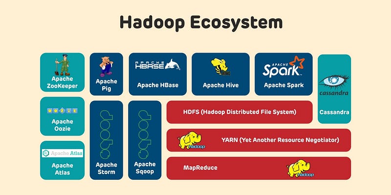
Hadoop

Hadoop HDFS

Hadoop Yarn

Hive

Zookeeper

Pig

Cassandra

Sqoop

Data Pipelines and WorkFlows

Data Pipelines

Transformation

Processing

Workflow

Monitoring

Airflow

DAG

Infrastructure

Docker

Docker vs Virtual Machines

Most important Docker commands

Kubernetes

Snowflake

Power BI

Power BI

Which chart to use and When?

Power BI — Data Analysis Expressions

Joins

Data Profiling

Cloud Data Engineering

Data Engineering on cloud

AWS

AWS Services

Google Cloud Platform

Google Cloud Platform services

Machine Learning Algorithms

Linear Regression

Logistic Regression

Decision Trees

Random Forest

Support Vector Machines

K Nearest Neighbors

K means Clustering

Hierarchical Clustering

Neural Networks

First we will cover how to explain above topics like a 5 year old and what each of these important concepts are —

• Scripting and Automation: Imagine you have a big toy collection and you want to clean and organize them every day. To save time, you can write a set of instructions (script) for your robot friend to follow, so it can clean and organize your toys automatically (automation). In a computer system, scripting and automation are used to automate repetitive tasks, saving time and improving efficiency.

Using the same analogy, Scripting and automation refer to the process of automating repetitive tasks and processes through scripting.

Here is an example of a scripting automation code in Python:

import time
import pyautogui

# Define the coordinates of the button to click
button_location = (100, 200)

# Define the number of times to click the button
num_clicks = 10

# Define the delay between clicks
delay = 1

# Automate the clicking of the button
for i in range(num_clicks):
    pyautogui.click(button_location)
    time.sleep(delay)

This code automates the clicking of a button on the screen using the PyAutoGUI library. It clicks the button at the specified location num_clicks times with a delay of 1 second between clicks.

• Shell Scripting: Imagine you want your robot friend to follow specific instructions to clean and organize your toy collection. To do that, you can write those instructions in a language that the robot understands (shell scripting).

Using the same analogy, Shell scripting is a type of scripting that allows you to automate tasks in a UNIX shell environment.

Here is an example of a scripting code in Python to automate a task:

import os

# Define the directory to work with
dir = '/path/to/directory'

# Iterate over all files in the directory
for filename in os.listdir(dir):
    # Get the full path of each file
    file_path = os.path.join(dir, filename)

    # Check if the file is a text file
    if file_path.endswith('.txt'):
        # Open the file and read its content
        with open(file_path, 'r') as file:
            content = file.read()

        # Modify the content of the file
        content = content.replace('old_string', 'new_string')

        # Write the modified content back to the file
        with open(file_path, 'w') as file:
            file.write(content)

This code iterates over all the files in a directory and performs some operations on the text files. It opens each text file, reads its content, modifies the content, and writes the modified content back to the file.

ETL (Extract, Transform, Load): Imagine you have toy collections at different friends’ houses and you want to combine them into one big collection. To do that, you first need to extract the toys from each friend’s house, transform them into a common format, and then load them into your big collection. In a computer system, ETL is a process to combine data from different sources into a single database or data warehouse.

Using the same analogy, ETL (Extract, Transform, Load) is a process used to extract data from various sources, transform the data into a desired format and load it into a target database. It is important because it helps to clean, standardize and integrate data from different sources into a central location for analysis and reporting.

Here is a basic example of an Extract, Transform, Load (ETL) code in Python using the Pandas library:

import pandas as pd

# Extract data from source (e.g. csv file)
df = pd.read_csv("data.csv")

# Transform data
df = df.rename(columns={'old_column_name': 'new_column_name'})
df = df[df['column_name'] > value]

# Load data into destination (e.g. database)
df.to_sql('table_name', con=engine, if_exists='replace', index=False)

This code extracts data from a csv file, performs some transformations on the data (renaming a column and filtering), and loads the transformed data into a database table.

• Relational Databases and SQL: Imagine you have a big toy collection and you want to keep track of all your toys, such as the type, color, and location of each toy. To do that, you can use a special tool (relational database) to store the information about each toy and write instructions (SQL) to retrieve and manipulate the information.

Using the same analogy, Relational databases use the SQL (Structured Query Language) to manage data stored in tables with rows and columns. SQL is used to insert, update, and retrieve data from a relational database.

• NoSQL Data Bases and Map Reduce: Imagine you have a big toy collection and you want to find all the toys that are blue. To do that, you can use a special tool (NoSQL database) that allows you to quickly search for toys based on their color. Map Reduce is a technique used to process large amounts of data in a distributed manner.

Using the same analogy, NoSQL databases, on the other hand, use a variety of data models, including key-value, document-based, graph, and columnar, to store and manage unstructured or semi-structured data. MapReduce is a programming model for processing large data sets that involves mapping data into key-value pairs and then reducing the data based on the keys.

Here is an example of a MapReduce program in Python using the mrjob library:

from mrjob.job import MRJob

class WordCount(MRJob):

    def mapper(self, _, line):
        for word in line.split():
            yield word.lower(), 1

    def reducer(self, word, counts):
        yield word, sum(counts)

if __name__ == '__main__':
    WordCount.run()

In this example, a MapReduce program is implemented as a class that inherits from the MRJob class of the mrjob library. The mapper method takes a line of text as input and splits it into words. For each word, the mapper method emits a key-value pair, where the key is the word in lowercase and the value is 1.

The reducer method takes a word as a key and a list of counts as values. The reducer method sums up the counts for each word and emits a key-value pair, where the key is the word and the value is the total count.

The MapReduce program can be run from the command line by executing the script. The mrjob library takes care of the underlying details of the MapReduce processing, such as parallelization, shuffling, and sorting.

• Data Warehouses and Data Lakes: Imagine you have a big toy collection and you want to store all the information about your toys in a single place. To do that, you can use a special storage (data warehouse or data lake) that allows you to store and access all your toy information easily.

Using the same analogy, Data Warehouses and Data Lakes are large centralized repositories for storing big data in a structured or semi-structured format for analysis and reporting. Structured data refers to data that is organized into tables with defined columns and relationships, while unstructured data refers to data that has no pre-defined format or structure, such as text or images.

Here is an example of how to read and write data to a data lake using the Apache Spark library in Python:

from pyspark.sql import SparkSession

# Create a Spark session
spark = SparkSession.builder.appName("DataLakeExample").getOrCreate()

# Read data from a data lake into a Spark DataFrame
df = spark.read.format("csv").option("header", "true").load("s3a://bucket_name/data.csv")

# Perform transformations on the DataFrame
df = df.filter(df['column_name'] > value)

# Write the transformed DataFrame back to the data lake
df.write.format("parquet").mode("overwrite").option("compression", "snappy").save("s3a://bucket_name/transformed_data")

# Stop the Spark session
spark.stop()

This code reads data from a data lake in the form of a csv file stored in an Amazon S3 bucket. It performs transformations on the data and writes the transformed data back to the data lake in the form of a parquet file. The compressed format used for the parquet file is Snappy.

• Data Visualization: Imagine you want to show your friends your big toy collection and how it has grown over time. To do that, you can use special tools (data visualization) to create graphs, charts, and images to represent the information about your toy collection.

Using the same analogy, Data visualization is the process of representing data, information, or insights in a graphical or pictorial format, such as charts, graphs, or maps. It helps people to understand and interpret complex data sets by making patterns and relationships between data points more recognizable and understandable.

Data visualization works by taking data and transforming it into a visual format. A software or tool is used to generate the visual representation based on the data, and various methods such as bar charts, line charts, and scatter plots are used to represent the data. The visual representation helps users to quickly see patterns, relationships, and outliers in the data, making it easier to understand and draw insights from the data.

Here is an example of how to create a basic line chart using the Matplotlib library in Python:

import matplotlib.pyplot as plt

# Define the data to be plotted
x = [1, 2, 3, 4, 5]
y = [2, 4, 1, 5, 3]

# Plot the line chart
plt.plot(x, y)

# Add labels and title to the chart
plt.xlabel('X-axis')
plt.ylabel('Y-axis')
plt.title('Line Chart Example')

# Show the chart
plt.show()

This code creates a line chart with the given data. It labels the x and y axis, adds a title to the chart, and finally displays the chart.

• Pandas and Numpy are like big helpers for people who work with lots and lots of numbers. Think of it like a big kitchen, and Pandas and Numpy are like two big chefs who help you cook the yummy numbers. They help you organize the numbers and make it easier for you to find what you’re looking for. And they can also help you make new dishes with the numbers, like counting how many there are and finding the average. It’s like magic for numbers!

Using the same analogy, Pandas and Numpy are popular data analysis libraries in Python. Pandas is used for data cleaning, manipulation and analysis, while Numpy is used for numerical computation and data manipulation.

Here is an example of how to use Pandas and Numpy in Python to perform data manipulation and analysis:

import pandas as pd
import numpy as np

# Create a Pandas DataFrame
data = {'column_1': [1, 2, 3, 4, 5], 'column_2': [2, 4, 1, 5, 3]}
df = pd.DataFrame(data)

# Use Numpy to calculate the mean of the values in column_1
mean = np.mean(df['column_1'])

# Add a new column to the DataFrame with the result of a calculation using existing columns
df['column_3'] = df['column_1'] + df['column_2']

# Use Pandas to group the data by values in column_1
grouped = df.groupby(['column_1'])

# Use Pandas to calculate the mean of each group
grouped_mean = grouped.mean()

This code creates a Pandas DataFrame from a dictionary, calculates the mean of the values in one of its columns using Numpy, adds a new column to the DataFrame with the result of a calculation using existing columns, groups the data by values in one of its columns, and calculates the mean of each group.

• Data Processing Techniques: Imagine you have a big toy collection and you want to process all the information about your toys. To do that, you can use different techniques such as batch processing or stream processing.

Using the same analogy, Data Pre-processing is the process of preparing data for use in a machine learning model or analysis. It includes tasks such as handling missing values, cleaning data, transforming data, and scaling data. Handling missing values is the process of dealing with missing or incomplete data in a dataset. This can include techniques such as mean/mode/median imputation, hot deck imputation, and regression imputation.

Here is an example of a data processing code in Python using Pandas:

import pandas as pd

# Load the data into a Pandas DataFrame
df = pd.read_csv('data.csv')

# Remove any rows with missing values
df.dropna(inplace=True)

# Filter the data to include only specific rows
df = df[df['column_name'] == 'value']

# Convert a column from string to numerical data type
df['column_name'] = pd.to_numeric(df['column_name'])

# Group the data by values in a column and calculate the mean of each group
grouped = df.groupby(['column_name'])
grouped_mean = grouped.mean()

# Write the processed data to a new file
grouped_mean.to_csv('processed_data.csv', index=False)

This code loads a csv file into a Pandas DataFrame, removes any rows with missing values, filters the data to include only specific rows, converts a column from a string to a numerical data type, groups the data by values in a column, calculates the mean of each group, and writes the processed data to a new file.

• Data cleaning is like cleaning up your room. Just like you pick up toys and put them in the right place, data cleaning is about making sure that information is organized and tidy. This helps make it easier to understand and use.

Using the same analogy, “Data Cleaning” refers to the process of identifying and removing errors, inconsistencies, and inaccuracies from a dataset. Mean/mode/median imputation refers to techniques used to replace missing values with the mean, mode, or median of the existing values in a dataset.

• Hot deck imputation refers to a technique used to replace missing values with values from similar records in a dataset.
• Rescale Data refers to the process of transforming data to be on the same scale, such as by scaling data to have a minimum and maximum value.
• Binarize Data refers to the process of converting data into binary values, such as converting continuous values into categorical values.
• Regression Imputation refers to a technique used to replace missing values with values predicted by a regression model.
• Stochastic regression imputation refers to a variation of regression imputation that uses random sampling in the regression model.
• Feature Scaling refers to the process of transforming data to be on the same scale, such as by scaling data to have a minimum and maximum value or mean and standard deviation.
• Data Augmentation refers to the process of creating additional data from existing data, such as rotating images to create new examples for image classification. Read and Process Large Datasets refers to the process of reading, processing, and analyzing large amounts of data, often using tools such as Pandas and Numpy.
• Data Profiling refers to the process of summarizing and exploring the properties of a dataset, such as the distribution of values and the presence of missing or outliers. Summary Functions refers to functions used to summarize data, such as calculating the mean, median, or standard deviation of a dataset.

Here is an example of data cleaning code in Python using Pandas:

import pandas as pd

# Load the data into a Pandas DataFrame
df = pd.read_csv('data.csv')

# Remove any rows with missing values
df.dropna(inplace=True)

# Remove duplicates
df.drop_duplicates(inplace=True)

# Replace any incorrect values with NaN
df.replace(0, np.nan, inplace=True)

# Fill missing values with the mean of the column
df.fillna(df.mean(), inplace=True)

# Write the cleaned data to a new file
df.to_csv('cleaned_data.csv', index=False)

This code loads a csv file into a Pandas DataFrame, removes any rows with missing values, removes duplicates, replaces incorrect values with NaN, fills missing values with the mean of the column, and writes the cleaned data to a new file.

• Big Data: Imagine you have a big toy collection and you have information about every toy in the world. To store and process all that information, you need special tools (big data) to handle the large volume, velocity, and variety of data.

Using the same analogy, Big data refers to extremely large and complex datasets that can’t be processed and analyzed by traditional data processing methods and tools. These datasets are generated by various sources, such as social media, internet of things (IoT) devices, and e-commerce platforms. Big data can come in various forms, including structured data (e.g., databases), semi-structured data (e.g., XML and JSON), and unstructured data (e.g., text, images, and videos).

Big data works by processing and analyzing extremely large datasets using specialized technologies and tools. Here are the general steps involved in processing big data:

1. Data Collection: The first step is to collect the data from various sources such as sensors, social media, and e-commerce platforms. The data can be stored in various formats, including structured, semi-structured, and unstructured data.
2. Data Storage: The next step is to store the data in a manner that enables efficient processing and analysis. Distributed file systems such as Hadoop HDFS and NoSQL databases like MongoDB and Cassandra are commonly used to store big data.
3. Data Processing: The third step is to process the data to make it ready for analysis. This can involve cleaning and transforming the data, as well as reducing its size. Technologies such as Apache Spark and Apache Storm are commonly used for big data processing.
4. Data Analysis: The fourth step is to analyze the processed data to extract insights and meaningful information. This can involve using statistical methods, machine learning algorithms, and data visualization tools.
5. Data Visualization: The final step is to present the results of the analysis in a way that is easily understood by humans. Data visualization tools such as Tableau and PowerBI are commonly used to create interactive dashboards and graphs that highlight key insights and trends in the data.

Here is an example of processing big data in Python using the pyspark library:

from pyspark import SparkContext
from pyspark.sql import SparkSession

# Create a Spark context and Spark session
sc = SparkContext('local', 'big data example')
spark = SparkSession(sc)

# Load the data into a Spark DataFrame
df = spark.read.csv('big_data.csv', header=True, inferSchema=True)

# Perform some data processing operations
df_processed = df.filter(df['column1'] > 100) \
                 .groupBy(df['column2']) \
                 .agg({'column3': 'mean'})

# Save the processed data
df_processed.write.parquet('processed_data.parquet')

# Stop the Spark context
sc.stop()

In this example, a Spark context and Spark session are created using the SparkContext and SparkSession classes from the pyspark library. The data is loaded into a Spark DataFrame using the read.csv method, and some data processing operations are performed using the filter, groupBy, and agg methods. The processed data is then saved using the write.parquet method, and the Spark context is stopped using the stop method.

• Data Pipelines and Workflows: Imagine you have a big toy collection and you want to make sure the toys are cleaned, organized, and stored properly every day. To do that, you can create a series of tasks (data pipeline) that need to be performed in a specific order (workflow) to make sure the toys are properly taken care of.

Using the same analogy, Data pipelines and workflows are processes that help manage the flow of data in an organization. A data pipeline is a series of steps that move data from one place to another. This helps ensure that the data is processed, transformed, and stored in a way that makes it useful and accessible to different people and systems.

A workflow is a set of tasks and processes that are automated in a specific order. Workflows help manage and automate the flow of data through a data pipeline. This includes tasks like cleaning, transforming, and analyzing data, as well as storing and delivering the results to different stakeholders.

Together, data pipelines and workflows help make sure that data is processed and delivered to the right people and systems in a timely and efficient manner.

Here is an example of building a data pipeline in Python using the scikit-learn library:

import pandas as pd
import numpy as np
from sklearn.pipeline import Pipeline
from sklearn.preprocessing import StandardScaler
from sklearn.impute import SimpleImputer
from sklearn.ensemble import RandomForestRegressor

# Load the data
data = pd.read_csv('data.csv')

# Define the steps in the pipeline
steps = [
    ('imputer', SimpleImputer(strategy='mean')),
    ('scaler', StandardScaler()),
    ('regressor', RandomForestRegressor(random_state=0))
]

# Create the pipeline
pipeline = Pipeline(steps)

# Split the data into features and target
X = data.drop('target', axis=1)
y = data['target']

# Fit the pipeline to the data
pipeline.fit(X, y)

# Predict using the pipeline
y_pred = pipeline.predict(X)

In this example, a data pipeline is created using the Pipeline class from the scikit-learn library. The pipeline consists of three steps: imputation of missing values using the SimpleImputer class, scaling of the data using the StandardScaler class, and fitting a RandomForestRegressor to the data. The pipeline is fit to the data using the fit method, and predictions can be made using the predict method.

• Infrastructure: Imagine you have a big toy collection and you want to make sure it’s protected and accessible to you and your friends. To do that, you can use special tools like Docker and Kubernetes to manage and protect your toy collection.

Using the same analogy, Infrastructure in big data refers to the hardware and software systems that support the storage, processing, and analysis of large and complex datasets. This infrastructure must be designed to handle the scale, variety, and velocity of big data, as well as ensure the reliability, security, and performance of big data applications. Examples of big data infrastructure include cloud computing platforms like Amazon Web Services (AWS) or Google Cloud Platform (GCP), large-scale data storage systems like Hadoop HDFS or Apache Cassandra, and big data processing frameworks like Apache Spark or Apache Flink.

• Cloud Data Engineering: Imagine you have a big toy collection and you want to store it in a safe place that you and your friends can access from anywhere. To do that, you can use cloud services like AWS or Google Cloud Platform to store and access your toy collection.

Using the same analogy, Cloud Data Engineering is a field that involves designing, building, and maintaining data processing systems in the cloud. It involves using cloud computing technologies, such as Amazon Web Services (AWS) or Google Cloud Platform (GCP), to store, process, and analyze large amounts of data. The goal is to make it easier to access, process, and manage data in a scalable and cost-effective manner. Cloud Data Engineering includes tasks such as setting up cloud-based data storage systems, designing data processing workflows, and creating automated systems for processing and analyzing data.

• Machine learning is like playing with toys to make the computer smarter. There are many different toys to play with and each one can help the computer learn different things.

Using the same analogy, Machine learning is a type of computer program that can learn and make predictions or decisions without being explicitly programmed to do so. It works by analyzing data and finding patterns in that data. Then, based on those patterns, the machine learning model can make predictions about future data. For example, a machine learning model could look at lots of pictures of animals and learn to identify different types of animals in new pictures, even ones it hasn’t seen before. The more data the model has, the better it becomes at making predictions.

• Linear Regression is like finding a straight line that best fits a bunch of points. The computer tries to use this line to make predictions about new points.

Using the same analogy, Linear Regression is a statistical method used to model the relationship between a dependent variable and one or more independent variables. Multi Linear Regression is an extension of linear regression that models the relationship between a dependent variable and multiple independent variables.

Polynomial Regression: A regression analysis in which the relationship between the independent variable x and the dependent variable y is modeled as an nth degree polynomial.

Support Vector Regression: A type of regression analysis that uses support vectors, or the points closest to the boundary between classes, to make predictions.

Decision Tree Regression: A regression analysis method based on decision trees, a type of machine learning algorithm used for classification and regression tasks.

Random Forest Regression: An ensemble learning method that combines multiple decision tree regressions to produce a more accurate prediction.

Here is an example of linear regression implementation in Python using the scikit-learn library:

import numpy as np
import matplotlib.pyplot as plt
from sklearn.datasets import make_regression
from sklearn.linear_model import LinearRegression

# Generate random regression data
X, y = make_regression(n_features=1, random_state=0)

# Train the linear regression model
reg = LinearRegression().fit(X, y)

# Plot the data
plt.scatter(X, y)

# Plot the regression line
plt.plot(X, reg.predict(X), color='red')
plt.xlabel('Feature')
plt.ylabel('Target')
plt.show()

In this example, random regression data is generated using the make_regression function from the scikit-learn library. The LinearRegression class from the scikit-learn library is used to train the linear regression model on the generated data. The data points are plotted using a scatter plot, and the regression line is plotted using a line plot.

• Logistic Regression is like trying to figure out the answer to a yes/no question based on a bunch of clues.

Using the same analogy, Logistic Regression is a statistical method for analyzing a dataset in which there are one or more independent variables that determine an outcome. The outcome is measured with a dichotomous variable (in which there are only two possible outcomes). It is used to predict a binary outcome (1 / 0, Yes / No, True / False) based on one or several predictor variables (features). It gives the probability of an event occurring based on the calculated coefficients of the independent variables. It is used in fields such as finance, medicine, psychology, and marketing to identify patterns and make predictions.

Logistic regression works by using an equation to model the relationship between the dependent binary variable and one or more independent variables (predictors). The equation is represented by a logistic curve (also known as the sigmoid function), which is used to model the probability of the dependent variable being 1.

The logistic regression equation takes the form of:

P(Y=1) = 1 / (1 + e^-(B0 + B1X1 + B2X2 + … + BnXn))

where:

• P(Y=1) is the probability of the dependent variable being 1
• B0 is the intercept term
• B1 to Bn are the coefficients for the predictor variables X1 to Xn
• e^-(B0 + B1X1 + B2X2 + … + BnXn) is the log odds

The coefficients are estimated using maximum likelihood estimation, which is a method for finding the values of the coefficients that maximize the likelihood of observing the data.

Once the coefficients are estimated, they can be used to make predictions about the dependent variable based on new data. The prediction is made by plugging in the values of the predictors into the equation and calculating the probability of the dependent variable being 1. If the probability is greater than 0.5, the prediction is 1; if it is less than 0.5, the prediction is 0.

Here is an example of logistic regression implementation in Python using the scikit-learn library:

import numpy as np
import matplotlib.pyplot as plt
from sklearn.datasets import make_classification
from sklearn.linear_model import LogisticRegression

# Generate random binary classification data
X, y = make_classification(n_features=2, random_state=0)

# Train the logistic regression model
clf = LogisticRegression()
clf.fit(X, y)

# Plot the decision boundary
x_min, x_max = X[:, 0].min() - 1, X[:, 0].max() + 1
y_min, y_max = X[:, 1].min() - 1, X[:, 1].max() + 1
xx, yy = np.meshgrid(np.arange(x_min, x_max, 0.1),
                     np.arange(y_min, y_max, 0.1))
Z = clf.predict(np.c_[xx.ravel(), yy.ravel()])
Z = Z.reshape(xx.shape)
plt.contourf(xx, yy, Z, cmap=plt.cm.RdYlBu, alpha=0.5)

# Plot the points
plt.scatter(X[:, 0], X[:, 1], c=y, cmap=plt.cm.RdYlBu)
plt.xlabel('Feature 1')
plt.ylabel('Feature 2')
plt.show()

In this example, random binary classification data is generated using the make_classification function from the scikit-learn library. The LogisticRegression class from the scikit-learn library is used to train the logistic regression model on the generated data. The decision boundary is plotted using a contour plot, and the points are plotted using a scatter plot, with the color of the points indicating the class label.

• Decision Trees are like a flowchart. The computer asks a bunch of questions to figure out what the answer is.

Using the same analogy, a decision tree is a type of algorithm used in machine learning for predictive modeling. It is a tree-like model of decisions and their possible consequences, expressed in a flowchart-like structure. Each internal node of the tree represents a “test” on an attribute (e.g. whether a coin flip comes up heads), each branch represents the outcome of the test, and each leaf node represents a class label (decision taken after computing all attributes).

The topmost node in the tree is known as the root node and the bottommost nodes are the terminal nodes or leaf nodes. A decision tree works by recursively splitting the data into subsets based on the most significant input feature until all the data in the subsets belong to the same class or a stopping criterion is reached. The final result is a tree-like representation of all possible decisions and their consequences. The goal of the decision tree is to minimize the prediction error rate, meaning that the tree is constructed such that each internal node results in a split of the data that makes it easier to predict the target variable.

Decision trees are widely used for both classification and regression tasks, as well as for feature selection and dimensionality reduction. They are easy to interpret, simple to build and fast to classify unseen data.

A decision tree works by recursively dividing the data into subsets based on the values of the input features. The process starts at the root node, where all the data is considered as a single group. Then, the algorithm selects the feature that results in the most significant split of the data. The data is then divided into smaller subsets based on the values of this feature, and each subset is assigned to a child node. This process continues until a stopping criterion is met, such as all data belonging to the same class or reaching a maximum depth of the tree.

Here’s a step-by-step explanation of how a decision tree works:

1. Select the best feature: The algorithm selects the feature that results in the best split of the data into smaller subsets. The best split is typically determined by measuring the impurity of the data in each subset, using metrics such as information gain, gain ratio, or Gini impurity.
2. Create internal nodes: The selected feature is used to create an internal node that splits the data into subsets. The internal node is labeled with the name of the feature and the conditions that determine the split.
3. Create child nodes: Each subset is assigned to a child node of the internal node. If the subset is pure, meaning that all data belongs to the same class, the child node is a leaf node. Otherwise, the process continues recursively with the child node as the root.
4. Repeat until stopping criterion met: The process continues until a stopping criterion is met, such as all data belonging to the same class or reaching a maximum depth of the tree.
5. Make predictions: Once the decision tree is built, it can be used to make predictions for new data. To make a prediction, the algorithm follows the path from the root to a leaf node, making decisions based on the conditions at each internal node. The prediction is the class label assigned to the reached leaf node.

Here is an example of decision tree implementation in Python using the scikit-learn library:

import numpy as np
import matplotlib.pyplot as plt
from sklearn.datasets import load_iris
from sklearn.tree import DecisionTreeClassifier

# Load the iris dataset
iris = load_iris()
X = iris.data[:, :2]  # we only take the first two features for visualization
y = iris.target

# Train the decision tree classifier
clf = DecisionTreeClassifier()
clf.fit(X, y)

# Plot the decision boundary
x_min, x_max = X[:, 0].min() - 1, X[:, 0].max() + 1
y_min, y_max = X[:, 1].min() - 1, X[:, 1].max() + 1
xx, yy = np.meshgrid(np.arange(x_min, x_max, 0.1),
                     np.arange(y_min, y_max, 0.1))
Z = clf.predict(np.c_[xx.ravel(), yy.ravel()])
Z = Z.reshape(xx.shape)
plt.contourf(xx, yy, Z, cmap=plt.cm.RdYlBu, alpha=0.5)

# Plot the points
plt.scatter(X[:, 0], X[:, 1], c=y, cmap=plt.cm.RdYlBu)
plt.xlabel('Sepal length')
plt.ylabel('Sepal width')
plt.show()

In this example, the iris dataset is loaded using the load_iris function from the scikit-learn library. The DecisionTreeClassifier class is used to train the decision tree classifier on the first two features of the data. The decision boundary is plotted using a contour plot, and the points are plotted using a scatter plot, with the color of the points indicating the class label.

• Random Forest is like a group of decision trees working together.

Using the same analogy, Random Forest is an ensemble machine learning algorithm used for both classification and regression tasks. It combines multiple decision trees to produce a more accurate and stable prediction. The idea behind random forest is to randomly select a subset of the features and a subset of the training data to build each decision tree. The final prediction is made by averaging the predictions of all the trees in the forest, or by taking the majority vote for classification problems.

Random Forest is called “random” because the algorithm randomly selects a subset of features and a subset of training data for each tree. This randomization helps to reduce the overfitting problem and increases the diversity of the trees in the forest, which results in better generalization performance on unseen data. The randomization also helps to reduce the correlation between the trees, which makes the prediction of the random forest more robust and accurate.

Random Forest is a popular machine learning algorithm because it is relatively simple to use, it can handle both categorical and numerical features, and it can handle missing data. Additionally, Random Forest is not sensitive to the scaling of the data, so it does not require any preprocessing of the data.

The algorithm works as follows:

1. Select random subsets of the features and random subsets of the training data: The algorithm randomly selects a subset of the features and a subset of the training data for each decision tree in the forest. This randomization helps to reduce overfitting and increase the diversity of the trees in the forest.
2. Grow a decision tree from each subset: For each tree, the algorithm builds a decision tree using the selected subset of features and training data. The decision tree is built using a standard decision tree algorithm such as ID3, C4.5, or CART.
3. Make predictions: To make a prediction for a new instance, the algorithm inputs the instance into each tree in the forest and collects the predictions of all the trees.
4. Aggregate the predictions: For regression problems, the predictions of all the trees are averaged to produce the final prediction. For classification problems, the predictions of all the trees are combined using a majority vote. The class with the most votes is selected as the final prediction.

Here’s an example of how you can build a random forest in Python using the scikit-learn library:

import numpy as np
from sklearn.ensemble import RandomForestClassifier
from sklearn.datasets import load_iris
from sklearn.model_selection import train_test_split

# Load the iris dataset
iris = load_iris()
X = iris.data
y = iris.target

# Split the data into training and test sets
X_train, X_test, y_train, y_test = train_test_split(X, y, test_size=0.2, random_state=42)

# Train a random forest classifier
clf = RandomForestClassifier(n_estimators=100, random_state=42)
clf.fit(X_train, y_train)

# Evaluate the model on the test set accuracy = clf.score(X_test, y_test) print("Accuracy:", accuracy)

In this example, we first load the iris dataset using the load_iris function from the sklearn.datasets module. The iris dataset contains four features and three target classes.

Next, we split the data into training and test sets using the train_test_split function.

After that, we train a random forest classifier using the RandomForestClassifier class from the sklearn.ensemble module. We set the n_estimators parameter to 100 to specify the number of trees in the forest. We also set the random_state parameter to 42 to make the results reproducible.

Finally, we evaluate the accuracy of the model on the test set using the score method. The score method returns the mean accuracy of the model on the given test data and labels.

• Support Vector Machines are like trying to draw a line to separate different groups of points.

Using the same analogy, Support Vector Machine (SVM) is a type of supervised learning algorithm used for classification and regression problems. It is a powerful and flexible machine learning algorithm that works by finding the best boundary that separates the data into different classes.

In SVM, the idea is to find the hyperplane (a line or a higher-dimensional plane) that best separates the data into different classes. The hyperplane that maximizes the margin, or the distance between the closest data points of each class, is selected as the best boundary. These closest data points are called support vectors and play a key role in determining the hyperplane.

SVM can handle both linear and non-linear data by transforming the data into a higher-dimensional space using a technique called kernel trick. In this transformed space, it becomes possible to find a linear boundary that separates the data into different classes.

Here’s an example of how you can build an SVM classifier in Python using the scikit-learn library:

import numpy as np
from sklearn import datasets
from sklearn.model_selection import train_test_split
from sklearn.svm import SVC

# Load the iris dataset
iris = datasets.load_iris()
X = iris.data
y = iris.target

# Split the data into training and test sets
X_train, X_test, y_train, y_test = train_test_split(X, y, test_size=0.2, random_state=42)

# Train a support vector machine classifier
clf = SVC(kernel='linear', C=1, random_state=42)
clf.fit(X_train, y_train)

# Evaluate the model on the test set
accuracy = clf.score(X_test, y_test)
print("Accuracy:", accuracy)

In this example, we first load the iris dataset using the load_iris function from the sklearn.datasets module. The iris dataset contains four features and three target classes.

Next, we split the data into training and test sets using the train_test_split function.

After that, we train an SVM classifier using the SVC class from the sklearn.svm module. We set the kernel parameter to 'linear' to specify that we want to use a linear SVM, and set the C parameter to 1 to specify the regularization parameter.

• K Nearest Neighbors is like asking your friends for their opinion. The computer looks at the k closest neighbors to a new point to figure out what it is.

Using the same analogy, Using the same analogy, KNN, or K-Nearest Neighbors, is a machine learning algorithm used for classification and regression. It works by finding the K nearest data points to a new observation and using the majority of the classifications (or the average value in regression) of those K points to make a prediction for the new observation.

In the case of classification, KNN classifies a new observation based on the majority vote of its K nearest neighbors. In the case of regression, KNN predicts the target value for a new observation based on the average value of its K nearest neighbors.

KNN is a simple, intuitive and fast algorithm, but it can also be sensitive to the scale of the data and to the choice of K. Nevertheless, it is widely used for a variety of applications and it’s a good starting point for getting familiar with machine learning.

Here is an example of KNN implementation in Python using scikit-learn library:

from sklearn.neighbors import KNeighborsClassifier

# Create a KNN classifier with 3 neighbors
knn = KNeighborsClassifier(n_neighbors=3)

# Train the classifier using the training data
knn.fit(X_train, y_train)

# Predict the class labels for the test data
y_pred = knn.predict(X_test)

# Evaluate the accuracy of the classifier
accuracy = knn.score(X_test, y_test)
print('Accuracy:', accuracy)

In this example, X_train and y_train are the features and target variables for the training data, and X_test and y_test are the features and target variables for the test data. The classifier is trained using the fit method, and the predictions are made using the predict method. The accuracy of the classifier is then evaluated using the score method.

Note that in this example, the number of neighbors (K) is set to 3. This is a hyperparameter that can be tuned to get the best performance for the specific dataset.

• K Means Clustering is like sorting toys into groups. The computer sorts points into k different groups based on their similarities.

Using the same analogy, K-means clustering is an unsupervised machine learning technique used for partitioning a set of points into K clusters, where K is a positive integer specified by the user. The technique aims to minimize the sum of squared distances between the points and their respective cluster centroids, which are the mean of the points in each cluster.

The algorithm starts by randomly initializing the centroids, then repeatedly performs two steps: (1) assignment of each point to the nearest centroid, and (2) recalculation of the centroids as the mean of the points in each cluster. The process continues until convergence, which occurs when the centroids no longer change.

K-means clustering works by partitioning a set of points into K clusters, where K is a user-specified positive integer, in such a way as to minimize the sum of squared distances between each point and its assigned cluster centroid.

The algorithm starts with an initial set of K centroids, which can be randomly generated or specified by the user. The points are then assigned to their closest centroid based on the Euclidean distance between the points and centroids. The centroids are then recomputed as the mean of the points in each cluster. This process is repeated until convergence, which occurs when the centroids no longer change.

Here is an example of K-means clustering in Python using the scikit-learn library:

import numpy as np
import matplotlib.pyplot as plt
from sklearn.cluster import KMeans

# Generate random data
np.random.seed(0)
X = np.random.randn(100, 2)

# Fit the K-means model
kmeans = KMeans(n_clusters=3)
kmeans.fit(X)

# Plot the data and cluster centroids
plt.scatter(X[:, 0], X[:, 1], c=kmeans.labels_)
plt.scatter(kmeans.cluster_centers_[:, 0], kmeans.cluster_centers_[:, 1], marker='x', color='r')
plt.show()

In this example, a set of 100 random 2-dimensional points is generated and stored in the X variable. The KMeans class from the scikit-learn library is used to fit the K-means model to the data, with the number of clusters specified as 3. The data is then plotted using a scatter plot, with the points colored according to their cluster assignment, and the cluster centroids are plotted as red crosses.

• Hierarchical Clustering is like making a family tree of toys. The computer makes a tree of how the points are related to each other.

Using the same analogy, Hierarchical clustering is a type of clustering algorithm that creates a hierarchy of clusters, represented as a tree-like structure called a dendrogram. The dendrogram shows the relationships between the different clusters and how they are combined to form larger clusters.

There are two main types of hierarchical clustering: Agglomerative and Divisive. Agglomerative clustering starts with individual data points and combines them into successively larger clusters, until all data points belong to a single cluster. Divisive clustering starts with all data points in a single cluster and splits the cluster into smaller sub-clusters until each data point is in its own cluster.

Hierarchical clustering is useful when you have a large number of data points and you want to find a meaningful grouping or organization of the data. By looking at the dendrogram, you can choose the number of clusters that best captures the relationships between the data points. The final clusters can then be used for further analysis or for making predictions about new data points.

Here’s an example of hierarchical clustering in Python using the scikit-learn library:

import numpy as np
from sklearn.cluster import AgglomerativeClustering

# Sample data points
X = np.array([[1, 2], [1, 4], [1, 0], [4, 2], [4, 4], [4, 0]])

# Fit the model
agg_cluster = AgglomerativeClustering(n_clusters=2)
agg_cluster.fit(X)

# Predict the clusters
predictions = agg_cluster.labels_

print(predictions)
# Output: [0 0 0 1 1 1]

In this example, the AgglomerativeClustering class is used to fit the model to the data X. The number of clusters is specified as n_clusters=2. The fit method is used to fit the model to the data. The cluster assignments are stored in predictions.

• Neural Networks is like a brain. The computer uses a network of simple calculations to solve complex problems.

Using the same analogy, A neural network is a machine learning model inspired by the structure and function of the human brain. It is a type of artificial neural network that is designed to recognize patterns.

A neural network consists of multiple layers of neurons, with the input layer receiving raw data, and the output layer producing the final prediction. The intermediate layers, known as hidden layers, perform the complex computations required to transform the input into the desired output.

The neurons in a neural network are connected by pathways called synapses, which represent the strength of the connection between neurons. The strengths of these connections, known as weights, are initially set to random values, but are adjusted during the training process to minimize the error between the predicted and actual outputs.

During the training process, the neural network is presented with a large number of examples and the weights are adjusted to minimize the error between the predicted and actual outputs. This process is known as backpropagation and is done using a optimization algorithm, such as gradient descent.

Once trained, the neural network can make predictions by processing new inputs and passing the information through the network, updating the activations of each neuron until the final prediction is produced by the output layer.

Here is an example of a simple neural network implemented in Python using the Keras library:

import numpy as np
import keras
from keras.models import Sequential
from keras.layers import Dense

# Define the data
x_train = np.array([[0, 0], [0, 1], [1, 0], [1, 1]])
y_train = np.array([[0], [1], [1], [0]])

# Initialize the model
model = Sequential()

# Add layers to the model
model.add(Dense(16, input_dim=2, activation='relu'))
model.add(Dense(1, activation='sigmoid'))

# Compile the model
model.compile(loss='binary_crossentropy', optimizer='adam', metrics=['accuracy'])

# Train the model
model.fit(x_train, y_train, epochs=500, batch_size=1, verbose=0)

# Evaluate the model
scores = model.evaluate(x_train, y_train)
print("\n%s: %.2f%%" % (model.metrics_names[1], scores[1]*100))

In this example, the Sequential class is used to initialize the model. The add method is used to add two layers to the model: the first layer has 16 neurons with a rectified linear unit (ReLU) activation function, and the second layer has 1 neuron with a sigmoid activation function. The compile method is used to compile the model, specifying the loss function and optimizer. The model is trained using the fit method, and the accuracy of the model is evaluated using the evaluate method.

• Feature Engineering refers to the process of creating new features or modifying existing features in a dataset to better represent the data and improve the performance of a machine learning model.
• GroupBy Features involves grouping a dataset based on one or more features to aggregate the data and derive insights.
• Categorical and Numerical Features refer to the different types of variables in a dataset. Categorical features are variables that have a limited number of categories or values, while numerical features are variables that can have any value within a given range.
• Missing Value Analysis involves identifying and dealing with missing values in a dataset. This can include removing rows or columns with missing values, imputing missing values, or using statistical methods to estimate missing values.
• Fill the missing Values refers to the process of replacing missing values with estimated values.
• Unique Value Analysis involves identifying and analyzing unique values in a dataset.
• Univariate Analysis refers to the analysis of a single feature or variable in a dataset, while “Bivariate Analysis” refers to the analysis of the relationship between two features or variables. “Multivariate Analysis” refers to the analysis of the relationships among three or more features or variables.
• Correlation Analysis is a statistical method used to determine the relationship between two or more features or variables in a dataset.
• “Spearman’s ρ”, “Pearson’s r”, “Kendall’s τ”, “Cramér’s V (φc)” and “Phik (φk)” are different methods of measuring correlation between variables.
• Data Processing Techniques refers to the various methods used to process and analyze data.
• Batch Processing and Stream Processing are two common methods of data processing. Batch processing involves processing data in batches, while stream processing involves processing data as it arrives in real-time.
• Apache Spark is a fast and general-purpose cluster computing system for processing large-scale data.
• Apache Kafka is a distributed event streaming platform used for real-time data processing and handling high volume, high velocity data.

Here is an example of batch processing using Apache Spark to count the number of words in a text file:

from pyspark import SparkConf, SparkContext

# Configure Spark
conf = SparkConf().setMaster("local").setAppName("WordCount")
sc = SparkContext(conf = conf)

# Load the text file into an RDD
lines = sc.textFile("/path/to/textfile.txt")

# Split the lines into words and count the number of occurrences of each word
word_counts = lines.flatMap(lambda line: line.split(" ")) \
                   .map(lambda word: (word, 1)) \
                   .reduceByKey(lambda a, b: a + b)

# Store the results
word_counts.saveAsTextFile("/path/to/wordcount_results")

Here is an example of stream processing using Apache Spark to compute a running word count from a Kafka stream:

from pyspark.sql import SparkSession
from pyspark.sql.functions import explode
from pyspark.sql.functions import split

# Create a Spark session
spark = SparkSession \
    .builder \
    .appName("StructuredKafkaWordCount") \
    .getOrCreate()

# Read data from a Kafka topic
df = spark \
  .readStream \
  .format("kafka") \
  .option("kafka.bootstrap.servers", "localhost:9092") \
  .option("subscribe", "topic") \
  .load()

# Split the values into words
words = df.select(
    explode(
        split(df.value, " ")
    ).alias("word")
)

# Compute the word count
word_count = words.groupBy("word").count()

# Start the streaming query
query = word_count \
    .writeStream \
    .outputMode("complete") \
    .format("console") \
    .start()

query.awaitTermination()

Here is an example of a basic Apache Spark command to calculate the average of a list of numbers:

# Start the Spark shell
./bin/spark-shell

# Create an RDD from a list of numbers
val numbers = sc.parallelize(List(1, 2, 3, 4, 5))

# Calculate the average
val avg = numbers.mean()

# Print the result
println(s"The average is: $avg")

Here is an example of a basic Apache Kafka producer that sends messages to a topic:

from kafka import KafkaProducer

# Create a Kafka producer
producer = KafkaProducer(bootstrap_servers=["localhost:9092"])

# Send a message to a topic
producer.send("topic", b"Hello, world!")

# Wait for the message to be sent and delivery reports to be received
producer.flush()

• Data Pipelines refers to a set of processes for the efficient and automated movement of data from one place to another.
• Transformation in data pipelines refers to the process of converting data from one format to another or transforming it in some way to make it more usable or valuable.
• Processing in data pipelines refers to the operation of transforming data using algorithms or statistical models.
• Workflow in data pipelines refers to the sequence of tasks that must be performed to complete a data processing task, such as data extraction, transformation, and loading.
• Monitoring in data pipelines refers to the ongoing process of observing and assessing the performance and progress of a pipeline to ensure that it is working as expected.
• Airflow is an open-source platform for programmatically authoring, scheduling, and monitoring workflows.
• “DAG” stands for Directed Acyclic Graph, and is a term used to describe the structure of a workflow in Airflow. A DAG represents the tasks that need to be performed, and the dependencies between these tasks, in a graphical manner.

Here is an example code to demonstrate the creation of a data pipeline with transformations, processing, workflows, monitoring, Airflow, and Directed Acyclic Graphs (DAGs):

# Import required libraries
from airflow import DAG
from airflow.operators.python_operator import PythonOperator
from airflow.operators.dummy_operator import DummyOperator
from datetime import datetime, timedelta

# Define default_args for the DAG
default_args = {
    'owner': 'airflow',
    'depends_on_past': False,
    'start_date': datetime(2023, 1, 1),
    'email_on_failure': False,
    'email_on_retry': False,
    'retries': 1,
    'retry_delay': timedelta(minutes=5)
}

# Define the DAG
dag = DAG(
    'data_pipeline_example',
    default_args=default_args,
    description='Data pipeline example',
    schedule_interval=timedelta(hours=1),
    catchup=False
)

# Define a function to perform data transformation
def data_transformation(**kwargs):
    # Perform data transformation here
    pass

# Define a function to perform data processing
def data_processing(**kwargs):
    # Perform data processing here
    pass

# Create tasks for the DAG
start_task = DummyOperator(
    task_id='start',
    dag=dag
)

transform_task = PythonOperator(
    task_id='transform',
    python_callable=data_transformation,
    provide_context=True,
    dag=dag
)

process_task = PythonOperator(
    task_id='process',
    python_callable=data_processing,
    provide_context=True,
    dag=dag
)

end_task = DummyOperator(
    task_id='end',
    dag=dag
)

# Define the workflow
start_task >> transform_task >> process_task >> end_task

# Monitor the DAG with Airflow
# The DAG can be monitored and managed through the Airflow web UI

This example demonstrates a basic data pipeline with three tasks: data transformation, data processing, and end. The data transformation and data processing tasks are implemented as Python functions, and the workflow is defined as a sequence of tasks connected by the >> operator. The pipeline is scheduled to run every hour and monitored through the Airflow web UI.

• Docker is a platform for creating, deploying, and running containers, which are isolated units of software that can run on any operating system.

The most important Docker commands include:

1. docker run - runs a command in a new container.
2. docker start - starts one or more stopped containers.
3. docker stop - stops one or more running containers.
4. docker ps - lists the containers running on a system.
5. docker image - manages images.
6. docker network - manages networks.
7. docker volume - manages volumes.

• Kubernetes is an open-source system for automating the deployment, scaling, and management of containerized applications. It works by grouping containers that make up an application into logical units for easy management and discovery.
• Snowflake is a cloud-based data warehousing platform that provides a data lake, data warehousing, and data analytics services. It allows users to store, retrieve, and analyze large amounts of structured and semi-structured data in a single, secure, and scalable environment.
• Hadoop HDFS stands for Hadoop Distributed File System and is the primary storage system for Hadoop. It is a scalable, fault-tolerant, and distributable file system that stores data across multiple nodes in a Hadoop cluster.
• Hadoop YARN stands for Yet Another Resource Negotiator and is a resource management system for Hadoop. It is responsible for managing the allocation of resources such as CPU, memory, and storage across the nodes in a Hadoop cluster.
• Hive is a data warehousing and SQL-like query language for Hadoop. It provides an interface for querying and managing large datasets stored in HDFS using a SQL-like language called HiveQL.
• Zookeeper is a distributed coordination service for distributed systems. It is used by Hadoop to coordinate the activities of nodes in a Hadoop cluster and maintain configuration information.
• Pig is a high-level platform for creating MapReduce programs used with Hadoop. It provides a language called Pig Latin for expressing data analysis programs, which are then compiled into sequences of MapReduce operations.

Here is an example of a Hive script to calculate the average age of customers in a data table:

-- Create a Hive table from customer data stored in HDFS
CREATE EXTERNAL TABLE customers (
  id INT,
  first_name STRING,
  last_name STRING,
  birth_date STRING
)
ROW FORMAT DELIMITED
FIELDS TERMINATED BY ','
STORED AS TEXTFILE
LOCATION '/user/data/customers';

-- Calculate the average age of customers
SELECT AVG(YEAR(FROM_UNIXTIME(UNIX_TIMESTAMP())) - YEAR(FROM_UNIXTIME(UNIX_TIMESTAMP(birth_date)))) as average_age
FROM customers;

Here is an example of a Pig script to calculate the total number of customers from each state:

-- Load customer data from HDFS into Pig
customers = LOAD '/user/data/customers' USING PigStorage(',') AS (
  id:int,
  first_name:chararray,
  last_name:chararray,
  birth_date:chararray,
  state:chararray
);

-- Group customers by state and calculate the total number of customers
grouped_customers = GROUP customers BY state;
counted_customers = FOREACH grouped_customers GENERATE group, COUNT(customers);

-- Store the result in HDFS
STORE counted_customers INTO '/user/data/customers_by_state' USING PigStorage(',');

• Cassandra is a NoSQL database management system. It is highly scalable and provides high performance, making it an attractive option for large-scale data storage and retrieval.
• Sqoop is a tool for efficiently transferring bulk data between Apache Hadoop and structured data stores such as relational databases. It supports incremental imports, which allows new and updated data to be transferred between Hadoop and structured data stores in real-time.

Here is an example code to demonstrate the usage of ZooKeeper, Pig, Cassandra, and Sqoop:

# ZooKeeper
# Start ZooKeeper Server
./bin/zkServer.sh start

# Connect to ZooKeeper
./bin/zkCli.sh

# Stop ZooKeeper Server
./bin/zkServer.sh stop

# Pig
# Run a Pig script
pig -f script.pig

# Cassandra
# Connect to Cassandra
cqlsh

# Create a keyspace in Cassandra
CREATE KEYSPACE example
WITH REPLICATION = {
  'class': 'SimpleStrategy',
  'replication_factor': '1'
};

# Create a table in Cassandra
CREATE TABLE example.table (
  id int PRIMARY KEY,
  name text,
  age int
);

# Insert data into the table
INSERT INTO example.table (id, name, age)
VALUES (1, 'John', 30);

# Select data from the table
SELECT * FROM example.table;

# Sqoop
# Import data from RDBMS to HDFS
sqoop import \
--connect jdbc:mysql://localhost/db \
--username root \
--password password \
--table table \
--target-dir /user/hdfs/data

# Export data from HDFS to RDBMS
sqoop export \
--connect jdbc:mysql://localhost/db \
--username root \
--password password \
--table table \
--export-dir /user/hdfs/data \
--input-fields-terminated-by '\t'

Here is a simple example of a data pipeline using Hadoop, Hive, Pig, YARN, and Sqoop:

1. Collect Data: Use Sqoop to import customer data from a relational database into Hadoop HDFS.

sqoop import \
--connect jdbc:mysql://localhost/dbname \
--username user \
--password password \
--table customers \
--target-dir /user/data/customers

2. Clean Data: Use Pig to clean the data by removing missing values and handling duplicates.

customers = LOAD '/user/data/customers' USING PigStorage(',') AS (
    id:int,
    first_name:chararray,
    last_name:chararray,
    birth_date:chararray,
    address:chararray,
    city:chararray,
    state:chararray,
    zip:chararray
);

filtered_customers = FILTER customers BY id IS NOT NULL;

deduped_customers = DISTINCT filtered_customers;

STORE deduped_customers INTO '/user/data/clean_customers' USING PigStorage(',');

3. Transform Data: Use Hive to transform the data into a format suitable for analysis. This may involve transforming the data into a different structure, or transforming the values of columns.

CREATE EXTERNAL TABLE customers (
    id INT,
    first_name STRING,
    last_name STRING,
    birth_date STRING,
    address STRING,
    city STRING,
    state STRING,
    zip STRING
)
ROW FORMAT DELIMITED
FIELDS TERMINATED BY ','
STORED AS TEXTFILE
LOCATION '/user/data/clean_customers';

CREATE TABLE customers_transformed AS
SELECT id, first_name, last_name, from_unixtime(unix_timestamp(birth_date, 'yyyy-MM-dd'), 'yyyy') AS birth_year, address, city, state, zip
FROM customers;

4. Load Data: Load the transformed data into a data store such as a database or data warehouse.

5. Monitor Data: Monitor the data pipeline to ensure that it is working as expected and that the data is being loaded correctly.

6. Analyze Data: Use Hive and Pig to perform analysis and gain insights into your business.

7. Automate: Automate the entire process by creating a workflow using YARN. This will allow you to schedule the pipeline to run regularly and monitor its performance.

New Projects Coming Soon!!

That’s it for now. Keep checking this post every day to see new projects.

Let me know if you have questions in the comment section below. Subscribe/ Follow, Like/Clap as it would encourage me to write more in my free time

Stay Tuned and Keep coding!!

Read More —

11 most important System Design Base Concepts

1. System design basics

2. Horizontal and vertical scaling

3. Load balancing and Message queues

4. High level design and low level design, Consistent Hashing, Monolithic and Microservices architecture

5. Caching, Indexing, Proxies

6. Networking, How Browsers work, Content Network Delivery ( CDN)

7. Database Sharding, CAP Theorem, Database schema Design

8. Concurrency, API, Components + OOP + Abstraction

9. Estimation and Planning, Performance

10. Map Reduce, Patterns and Microservices

11. SQL vs NoSQL and Cloud

12. Most Popular System Design Questions

13. System Design Template — How to solve any System Design Question

14. Quick RoundUp : Solved System Design Case Studies

System Design Case Studies — In Depth

Design Instagram

Design Netflix

Design Reddit

Design Amazon

Design Messenger App

Design Twitter

Design URL Shortener

Design Dropbox

Design Youtube

Design API Rate Limiter

Design Web Crawler

Design Amazon Prime Video

Design Facebook’s Newsfeed

Design Yelp

Design Uber

Design Tinder

Design Tiktok

Design Whatsapp

Most Popular System Design Questions

Mega Compilation : Solved System Design Case studies

Complete Data Structures and Algorithm Series

Complexity Analysis

Backtracking

Sliding Window

Greedy Technique

Two pointer Technique

Arrays

Linked List

Strings

Stack

Queues

Hash Table/Hashing

Binary Search

1- D Dynamic Programming

Divide and Conquer Technique

Recursion

Some of the other best Series —

60 days of Data Science and ML Series with projects

30 Days of Natural Language Processing ( NLP) Series

30 days of Machine Learning Ops

30 days of Data Structures and Algorithms and System Design Simplified

60 Days of Deep Learning with Projects Series

30 days of Data Engineering with projects Series

Data Science and Machine Learning Research ( papers) Simplified **

100 days : Your Data Science and Machine Learning Degree Series with projects

23 Data Science Techniques You Should Know

Tech Interview Series — Curated List of coding questions

Complete System Design with most popular Questions Series

Complete Data Visualization and Pre-processing Series with projects

Complete Python Series with Projects

Complete Advanced Python Series with Projects

Kaggle Best Notebooks that will teach you the most

Complete Developers Guide to Git

Exceptional Github Repos — Part 1

Exceptional Github Repos — Part 2

All the Data Science and Machine Learning Resources

210 Machine Learning Projects

Tech Newsletter —

If you are interested, you can join my newsletter through which I send tech interview tips, techniques, patterns, hacks — Software Development, ML, Data Science, Startups and Technology projects to more than 30K readers. You can subscribe to Tech Brew :

For Python Projects —

For complete 60 days of Data Science and ML : Day 1 — Day 60 : Quick Recap of 60 days of Data Science and ML

Follow for more updates.

For other projects, tune to —

Build Machine Learning Pipelines( With Code)

Recurrent Neural Network with Keras

Clustering Geolocation Data in Python using DBSCAN and K-Means

Facial Expression Recognition using Keras

Hyperparameter Tuning with Keras Tuner

Custom Layers in Keras