
Implemented Data Engineering Projects
Repo for all the projects ( vertical post)…
Welcome back peeps.
Since we are now focusing on our goals for 2023 — new vertical series than horizontal ( means you will find all the contents of the series in one post and projects in second than developing/extending it to new posts every time). So, keep checking this post every day to see new projects.
Prerequisite to these projects —
Complete 60 days of Data Science and Machine Learning before starting this series ( link below) —
Projects Videos —
All the projects, data structures, SQL, algorithms, system design, Data Science and ML , Data Analytics, Data Engineering, , Implemented Data Science and ML projects, Implemented Data Engineering Projects, Implemented Deep Learning Projects, Implemented Machine Learning Ops Projects, Implemented Time Series Analysis and Forecasting Projects, Implemented Applied Machine Learning Projects, Implemented Tensorflow and Keras Projects, Implemented PyTorch Projects, Implemented Scikit Learn Projects, Implemented Big Data Projects, Implemented Cloud Machine Learning Projects, Implemented Neural Networks Projects, Implemented OpenCV Projects,Complete ML Research Papers Summarized, Implemented Data Analytics projects, Implemented Data Visualization Projects, Implemented Data Mining Projects, Implemented Natural Leaning Processing Projects, MLOps and Deep Learning, Applied Machine Learning with Projects Series, PyTorch with Projects Series, Tensorflow and Keras with Projects Series, Scikit Learn Series with Projects, Time Series Analysis and Forecasting with Projects Series, ML System Design Case Studies Series videos will be published on our youtube channel ( just launched).
Subscribe today!
Tech Newsletter —
If you are interested, you can join my newsletter through which I send tech interview tips, techniques, patterns, hacks — Software Development, ML, Data Science, Startups and Technology projects to more than 35K readers. You can subscribe to Ignito:
Let’s dive in!
Data engineering is the process of designing, building, and maintaining the infrastructure and systems that support the acquisition, storage, and processing of data.
It involves the design and implementation of data pipelines, storage systems, and data processing frameworks that enable the data to be collected, stored, and made available for analysis and reporting.
Data engineers work closely with data scientists and analysts to understand the data needs and create the necessary infrastructure to support their work. They are responsible for ensuring that data is accurate, complete, and available in a timely manner.
Some of the key tasks and responsibilities of data engineers include:
- Designing and building data pipelines to extract data from various sources, including databases, APIs, and file systems, and transform it into a format that can be used for analysis.
- Building and maintaining data storage systems, including relational databases, NoSQL databases, and data warehousing solutions.
- Designing and implementing data processing frameworks, such as Apache Hadoop and Apache Spark, to enable large-scale data processing and analysis.
- Implementing data quality and data governance controls to ensure data accuracy and completeness.
- Monitoring and troubleshooting data pipeline and processing issues.
- Developing and maintaining documentation and metadata for data pipelines and storage systems.
- Collaborating with data scientists and analysts to understand their data needs and create the necessary infrastructure to support their work.
Data engineering is a crucial field in the big data ecosystem. It plays a key role in the development of data-driven systems and applications by providing the necessary infrastructure and tools to enable data scientists and analysts to extract insights from data.
This post will house all the Data Engineering projects related to the topics below-
Scripting and Automation
Relational Databases and SQL
NoSQL Data bases and Map Reduce
Data Analysis
Data Processing Techniques
Big Data
Data Pipelines and WorkFlows
Infrastructure
Power BI
Cloud Data Engineering
Machine Learning Algorithms
First we will cover all the above mentioned topics in detail with code implementation —
Scripting and Automation
Scripting and Automation are important components of Data Engineering, as they help to streamline the process of data collection, transformation, and analysis. In this answer, I will explain each stage of Scripting and Automation in Data Engineering, along with a Python implementation example.
Data Collection: The first step in any data engineering project is to collect the data. This can be done manually, but it is often more efficient to automate the process using scripts. Python has many libraries and tools for web scraping and data extraction. Here is an example of how to use the BeautifulSoup library to scrape data from a website:
import requests
from bs4 import BeautifulSoup
url = 'https://www.example.com'
response = requests.get(url)soup = BeautifulSoup(response.text, 'html.parser')
data = soup.find('div', {'class': 'data'}).textprint(data)This code sends a request to the URL and uses BeautifulSoup to parse the HTML. It then finds the div element with the class “data” and extracts the text. This data can then be saved to a file or uploaded to a database.
Data Transformation: After collecting the data, it often needs to be transformed to be more useful. This can include cleaning the data, converting it to a different format, or joining multiple datasets. Python has many libraries for data manipulation and transformation, such as Pandas. Here is an example of how to use Pandas to clean and transform a dataset:
import pandas as pddata = pd.read_csv('data.csv')
data = data.dropna() # remove rows with missing values
data['date'] = pd.to_datetime(data['date']) # convert date column to datetime format
data['total'] = data['quantity'] * data['price'] # create a new column for the total costdata.to_csv('transformed_data.csv', index=False) # save the transformed data to a fileThis code reads a CSV file into a Pandas dataframe and then cleans and transforms the data. It drops rows with missing values, converts the date column to datetime format, and creates a new column for the total cost. Finally, it saves the transformed data to a new CSV file.
Data Analysis: Once the data has been collected and transformed, it can be analyzed to gain insights and make decisions. Python has many libraries for data analysis and visualization, such as Matplotlib and Seaborn. Here is an example of how to use Matplotlib to create a bar chart of the total cost by product:
import pandas as pd
import matplotlib.pyplot as plt
data = pd.read_csv('transformed_data.csv')totals_by_product = data.groupby('product')['total'].sum()plt.bar(totals_by_product.index, totals_by_product.values)
plt.xlabel('Product')
plt.ylabel('Total Cost')
plt.show()This code reads the transformed data from the previous step and groups it by product to calculate the total cost. It then creates a bar chart using Matplotlib to visualize the results.
Automation: Finally, all of these steps can be automated using scripts to create a streamlined data engineering pipeline. This can include scheduling scripts to run at regular intervals, setting up triggers to run scripts when new data is available, or using cloud services like AWS Lambda to run scripts in response to events. Here is an example of how to use the Python package APScheduler to schedule a script to run every hour:
from apscheduler.schedulers.blocking import BlockingScheduler

def collect_data():
    # code to collect data

def transform_data():
    # code to transform data

def analyze_data():
    # code to analyze data

scheduler = BlockingScheduler()

scheduler.add_job(collect_data, 'interval', hours=1)
scheduler.add_job(transform_data, 'interval', hours=2)
scheduler.add_job(analyze_data, 'interval', hours=3)

scheduler.start()
This code imports the BlockingScheduler class from the apscheduler.schedulers module. It then defines three functions to collect, transform, and analyze the data. Finally, it creates a new scheduler object and adds three jobs to it using the add_job method. Each job is scheduled to run at a different interval, with collect_data running every hour, transform_data running every two hours, and analyze_data running every three hours. Finally, the start method is called to start the scheduler. This will run the jobs at the scheduled intervals until the program is stopped or interrupted.
Shell Scripting
Shell scripting is a powerful tool in data engineering that allows you to automate repetitive tasks, manipulate files and data, and perform system operations. The following are the stages of Shell scripting in data engineering:
- Planning and design
- Writing the code
- Testing and debugging
- Deployment and maintenance
Let’s implement each stage using Python.
Planning and design
The first step in shell scripting is to plan and design the script. This involves identifying the task to be automated and breaking it down into smaller steps. You should also identify the input and output data, and any dependencies or constraints.
Example task: Automate the process of downloading and processing a CSV file from a website.
Design:
- Download the CSV file from the website using Python requests module
- Store the CSV file locally
- Process the CSV file using Python Pandas module
- Generate a report based on the processed data
- Email the report to a specified email address
Writing the code
Once you have a design for the script, the next step is to write the code. In this stage, you’ll write the code to implement the steps identified in the planning and design stage.
Here’s an example code for our CSV file automation task:
#!/bin/bash
# Download the CSV file from the website using Python requests module
curl -o data.csv https://example.com/data.csv
# Store the CSV file locally
mv data.csv /path/to/local/folder# Process the CSV file using Python Pandas module
python process_csv.py /path/to/local/folder/data.csv# Generate a report based on the processed data
python generate_report.py /path/to/local/folder/data_processed.csv# Email the report to a specified email address
python send_email.py /path/to/local/folder/report.pdf [email protected]Testing and debugging
After writing the code, it’s important to test it to ensure it works as expected. This involves running the script and verifying that it produces the desired output.
Example test:
./process_data.sh
This will run the script and execute all the steps. You should verify that the CSV file is downloaded and stored locally, the CSV file is processed and a report is generated and emailed to the specified address.
If there are any issues, you should debug the code to identify and fix the problem.
Deployment and maintenance
Once the script is working correctly, you can deploy it to production. This involves copying the script to the production environment and scheduling it to run at a specified interval using a tool like Cron.
You should also perform maintenance on the script, such as updating it to handle changes in the input data or fixing bugs. This ensures that the script continues to work correctly over time.
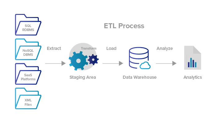
ETL ( Extract, Tranform and Load) basics
ETL (Extract, Transform, Load) is a process used in data engineering to extract data from various sources, transform it into a suitable format, and then load it into a target database or data warehouse. In this response, I will explain and implement each stage of the ETL process using Python.
Extract
The first stage of the ETL process is to extract data from various sources. The source data can be in various formats, such as CSV, Excel, XML, JSON, or SQL databases. Python has many libraries that can be used to extract data from these sources. Here’s an example of how to extract data from a CSV file using Python’s pandas library:
import pandas as pd# Extract data from CSV file
data = pd.read_csv('data.csv')Transform
The second stage of the ETL process is to transform the extracted data into a suitable format for the target database or data warehouse. This involves cleaning, filtering, merging, or aggregating the data as needed. Python has many libraries that can be used to transform data. Here’s an example of how to transform data by filtering and aggregating it using Python’s pandas library:
# Filter data
filtered_data = data[data['age'] > 30]
# Aggregate data
grouped_data = filtered_data.groupby(['gender'])['salary'].mean()Load
The final stage of the ETL process is to load the transformed data into a target database or data warehouse. Python has many libraries that can be used to load data into databases, such as psycopg2 for PostgreSQL and mysql-connector-python for MySQL. Here's an example of how to load data into a PostgreSQL database using Python's psycopg2 library:
import psycopg2# Connect to the database
conn = psycopg2.connect(
host="localhost",
database="mydb",
user="myuser",
password="mypassword"
)# Create a cursor
cur = conn.cursor()# Load data into a table
for index, row in grouped_data.iterrows():
cur.execute("INSERT INTO mytable (gender, avg_salary) VALUES (%s, %s)", (index, row['salary']))# Commit the transaction
conn.commit()# Close the cursor and connection
cur.close()
conn.close()In summary, the ETL process involves three stages: Extract, Transform, and Load. Python has many libraries that can be used to extract, transform, and load data, such as pandas for data manipulation, psycopg2 for database connections, and mysql-connector-python for MySQL connections.
ETL Tools
ETL tools typically consist of three main components:
- Extract: This involves collecting data from various sources such as databases, web services, or files.
- Transform: This involves cleaning, filtering, and transforming the data into a structured format that is easy to analyze or store.
- Load: This involves loading the transformed data into a data warehouse or other storage system.
ETL tools automate and streamline this process, making it faster, more efficient, and more accurate. They are essential for data engineering projects that involve large amounts of data from multiple sources.
Python is a popular language for data engineering and has many libraries and frameworks that can be used for ETL. Some of the commonly used libraries for data extraction are pandas, requests, and sqlalchemy. For data transformation, pandas, numpy, and datetime are commonly used. For loading data into various storage systems, pandas, sqlalchemy, and other specialized libraries can be used.
Implementation
Here is an example implementation of ETL tools in data engineering with Python:
import pandas as pd
import sqlalchemy
# Extract data from a database
engine = sqlalchemy.create_engine('postgresql://user:password@host:port/database')
query = "SELECT * FROM table"
data = pd.read_sql(query, engine)# Transform data by filtering rows and columns
filtered_data = data[data['age'] > 18][['name', 'age']]# Load data into a data warehouse
engine = sqlalchemy.create_engine('postgresql://user:password@host:port/database')
filtered_data.to_sql('filtered_table', engine, if_exists='replace', index=False)In this example, we extract data from a PostgreSQL database using the sqlalchemy library, transform the data by filtering rows and columns using pandas, and load the data into a PostgreSQL database using sqlalchemy.
Relational Databases and SQL
Relational databases are a type of database that organizes data into one or more tables with columns and rows. SQL (Structured Query Language) is the standard language used to communicate with relational databases.
Creating a Database
The first stage in relational databases is creating a database. A database is a collection of tables that contain data. In SQL, we can use the CREATE DATABASE statement to create a new database. Here is an example implementation using the sqlite3 module in Python:
import sqlite3# create a connection to the database
conn = sqlite3.connect('mydatabase.db')# create a cursor object
cursor = conn.cursor()# create a new database
cursor.execute('CREATE DATABASE mydatabase')Creating a Table
After creating a database, the next stage is creating a table. A table is a collection of related data organized into rows and columns. In SQL, we can use the CREATE TABLE statement to create a new table. Here is an example implementation using the sqlite3 module in Python:
import sqlite3# create a connection to the database
conn = sqlite3.connect('mydatabase.db')# create a cursor object
cursor = conn.cursor()# create a new table
cursor.execute('''
CREATE TABLE users
(id INTEGER PRIMARY KEY, name TEXT, age INTEGER, email TEXT)
''')Inserting Data
The next stage is inserting data into a table. In SQL, we can use the INSERT INTO statement to insert data into a table. Here is an example implementation using the sqlite3 module in Python:
import sqlite3# create a connection to the database
conn = sqlite3.connect('mydatabase.db')# create a cursor object
cursor = conn.cursor()# insert data into the users table
cursor.execute('''
INSERT INTO users (name, age, email)
VALUES ('John', 30, '[email protected]')
''')# commit the transaction
conn.commit()Updating Data
The next stage is updating data in a table. In SQL, we can use the UPDATE statement to update data in a table. Here is an example implementation using the sqlite3 module in Python:
import sqlite3# create a connection to the database
conn = sqlite3.connect('mydatabase.db')# create a cursor object
cursor = conn.cursor()# update data in the users table
cursor.execute('''
UPDATE users
SET age = 35
WHERE name = 'John'
''')# commit the transaction
conn.commit()Deleting Data
The final stage is deleting data from a table. In SQL, we can use the DELETE FROM statement to delete data from a table. Here is an example implementation using the sqlite3 module in Python:
import sqlite3# create a connection to the database
conn = sqlite3.connect('mydatabase.db')# create a cursor object
cursor = conn.cursor()# delete data from the users table
cursor.execute('''
DELETE FROM users
WHERE name = 'John'
''')# commit the transaction
conn.commit()In summary, relational databases and SQL are used to organize and manipulate data in tables with columns and rows. In Python, we can use various modules, such as sqlite3 and psycopg2, to interact with relational databases and perform SQL operations, such as creating databases and tables, inserting and updating data, and deleting data.
Basic SQL
Basic SQL (Structured Query Language) is a programming language used to communicate with relational databases.
Selecting Data
The first stage in basic SQL is selecting data from a table. We can use the SELECT statement to select data from one or more tables. Here is an example implementation using the sqlite3 module in Python:
import sqlite3# create a connection to the database
conn = sqlite3.connect('mydatabase.db')# create a cursor object
cursor = conn.cursor()# select all data from the users table
cursor.execute('SELECT * FROM users')# print the results
for row in cursor.fetchall():
print(row)Filtering Data
The next stage is filtering data from a table. We can use the WHERE clause to filter data based on one or more conditions. Here is an example implementation using the sqlite3 module in Python:
import sqlite3# create a connection to the database
conn = sqlite3.connect('mydatabase.db')# create a cursor object
cursor = conn.cursor()# select data from the users table where age is greater than 30
cursor.execute('SELECT * FROM users WHERE age > 30')# print the results
for row in cursor.fetchall():
print(row)Sorting Data
The next stage is sorting data from a table. We can use the ORDER BY clause to sort data based on one or more columns. Here is an example implementation using the sqlite3 module in Python:
import sqlite3# create a connection to the database
conn = sqlite3.connect('mydatabase.db')# create a cursor object
cursor = conn.cursor()# select data from the users table and sort by age in ascending order
cursor.execute('SELECT * FROM users ORDER BY age ASC')# print the results
for row in cursor.fetchall():
print(row)Joining Tables
The next stage is joining two or more tables together. We can use the JOIN clause to combine rows from two or more tables based on a related column. Here is an example implementation using the sqlite3 module in Python:
import sqlite3# create a connection to the database
conn = sqlite3.connect('mydatabase.db')# create a cursor object
cursor = conn.cursor()# join data from the users and orders tables based on the user_id column
cursor.execute('''
SELECT users.name, orders.product
FROM users
JOIN orders
ON users.id = orders.user_id
''')# print the results
for row in cursor.fetchall():
print(row)Aggregating Data
The final stage is aggregating data from a table. We can use aggregate functions, such as SUM, AVG, and COUNT, to perform calculations on a set of rows. Here is an example implementation using the sqlite3 module in Python:
import sqlite3# create a connection to the database
conn = sqlite3.connect('mydatabase.db')# create a cursor object
cursor = conn.cursor()# calculate the average age of the users
cursor.execute('SELECT AVG(age) FROM users')# print the result
print(cursor.fetchone()[0])In summary, basic SQL is a powerful tool for data engineering that allows us to select, filter, sort, join, and aggregate data in relational databases. In Python, we can use various modules, such as sqlite3 and psycopg2, to interact with relational databases and perform basic SQL operations.
Advanced SQL
Advanced SQL involves more complex queries that allow us to manipulate data in sophisticated ways. In this response, I will explain each stage of advanced SQL in data engineering and provide a Python implementation for each stage.
Subqueries
A subquery is a query nested inside another query. We can use subqueries to retrieve data from one or more tables based on the result of another query. Here is an example implementation using the sqlite3 module in Python:
import sqlite3# create a connection to the database
conn = sqlite3.connect('mydatabase.db')# create a cursor object
cursor = conn.cursor()# select data from the users table where age is greater than the average age
cursor.execute('''
SELECT name, age
FROM users
WHERE age > (
SELECT AVG(age)
FROM users
)
''')# print the results
for row in cursor.fetchall():
print(row)Window Functions
Window functions are used to perform calculations across a set of rows that are related to the current row. We can use window functions to calculate running totals, rankings, and moving averages. Here is an example implementation using the psycopg2 module in Python:
import psycopg2# create a connection to the database
conn = psycopg2.connect(
host="localhost",
database="mydatabase",
user="myusername",
password="mypassword"
)# create a cursor object
cursor = conn.cursor()# calculate the running total of sales by month
cursor.execute('''
SELECT month, sales, SUM(sales) OVER (ORDER BY month) AS running_total
FROM sales_data
''')# print the results
for row in cursor.fetchall():
print(row)Common Table Expressions
A common table expression (CTE) is a named temporary result set that can be referenced within a query. We can use CTEs to simplify complex queries and make them easier to read and maintain. Here is an example implementation using the psycopg2 module in Python:
import psycopg2# create a connection to the database
conn = psycopg2.connect(
host="localhost",
database="mydatabase",
user="myusername",
password="mypassword"
)# create a cursor object
cursor = conn.cursor()# define a CTE that calculates the total sales by product
cursor.execute('''
WITH total_sales AS (
SELECT product, SUM(sales) AS total
FROM sales_data
GROUP BY product
)
SELECT product, sales / total AS market_share
FROM sales_data
JOIN total_sales
ON sales_data.product = total_sales.product
''')# print the results
for row in cursor.fetchall():
print(row)Pivot Tables
A pivot table is a table that summarizes data by aggregating it across multiple dimensions. We can use pivot tables to transform data from a long format to a wide format. Here is an example implementation using the pandas module in Python:
import pandas as pd
import psycopg2
# create a connection to the database
conn = psycopg2.connect(
host="localhost",
database="mydatabase",
user="myusername",
password="mypassword"
)# read the sales data into a pandas DataFrame
df = pd.read_sql_query('SELECT * FROM sales_data', conn)# pivot the sales data by month and product
pivot_table = df.pivot_table(
index='month',
columns='product',
values='sales',
aggfunc='sum'
)# print the results
print(pivot_table)NoSQL Data bases and Map Reduce
NoSQL databases are a type of database that are designed to handle large volumes of unstructured and semi-structured data. MapReduce is a programming model for processing and generating large data sets with a parallel, distributed algorithm on a cluster. In this response, I will explain each stage of NoSQL databases and MapReduce in data engineering and provide a Python implementation for each stage.
NoSQL Databases
NoSQL databases can be broadly categorized into four types: document-based, key-value, column-family, and graph-based databases. Each type of database is optimized for a specific use case.
Document-based Databases
Document-based databases store data in a semi-structured format, such as JSON or XML. Data is stored in documents, which can contain nested data structures. Here is an example implementation using the pymongo module in Python to insert a document into a MongoDB database:
import pymongo# create a connection to the database
client = pymongo.MongoClient('mongodb://localhost:27017')# select the database and collection
db = client['mydatabase']
collection = db['mycollection']# insert a document into the collection
document = {'name': 'John', 'age': 30, 'address': {'city': 'New York', 'state': 'NY'}}
collection.insert_one(document)Key-value Databases
Key-value databases store data as a collection of key-value pairs. Each key is unique and maps to a value, which can be any type of data. Here is an example implementation using the Redis module in Python to set a key-value pair:
import redis# create a connection to the Redis server
r = redis.Redis(host='localhost', port=6379)# set a key-value pair
r.set('name', 'John')Column-family Databases
Column-family databases store data in column families, which are collections of columns that are stored together. Each column can have a different data type and can contain multiple values. Here is an example implementation using the Cassandra module in Python to insert data into a column-family database:
from cassandra.cluster import Cluster# create a connection to the database
cluster = Cluster(['localhost'])
session = cluster.connect()# create the keyspace and column family
session.execute('''
CREATE KEYSPACE mykeyspace
WITH replication = {'class': 'SimpleStrategy', 'replication_factor': 1}
''')session.execute('''
CREATE TABLE mytable (
id int,
name text,
age int,
PRIMARY KEY (id)
)
''')# insert data into the table
session.execute('''
INSERT INTO mytable (id, name, age)
VALUES (1, 'John', 30)
''')Graph-based Databases
Graph-based databases store data as nodes and edges, which are used to represent relationships between the nodes. Each node and edge can have multiple properties, which can be used to store additional information about the data. Here is an example implementation using the Neo4j module in Python to create a node and a relationship between two nodes:
from neo4j import GraphDatabase

# create a connection to the database
driver = GraphDatabase.driver('bolt://localhost:7687', auth=('neo4j', 'mypassword'))

# create a node
with driver.session() as session:
    result = session.run('CREATE (person:Person {name: $name, age: $age})', name='John', age=30)

# create a relationship between two nodes
with driver.session() as session:
    result = session.run('MATCH (a:Person), (b:Person) WHERE a.name = $name1 AND b.name = $name2 CREATE (a)-[r:KNOWS]->(b)', name1='John', name2='Jane')

# retrieve data from the database
with driver.session() as session:
    result = session.run('MATCH (a:Person)-[:KNOWS]->(b:Person) WHERE a.name = $name RETURN b.name', name='John')
    for record in result:
        print(record['b.name'])
Data Warehouses
Data Warehousing is the process of collecting, storing, and managing data from various sources to support business intelligence (BI) analysis and reporting. Data Warehousing involves several stages including data extraction, transformation, loading, and querying. Here’s a brief explanation and implementation of each stage using Python:
Data Extraction: Data extraction is the process of retrieving data from various sources such as databases, applications, and files. In data warehousing, data is extracted from multiple sources and consolidated into a single data repository. Python has many libraries for data extraction, such as Pandas, which can be used to extract data from databases, CSV files, and Excel files.
Example:
import pandas as pd# extract data from CSV file
data = pd.read_csv('data.csv')# extract data from SQL database
import sqlite3
connection = sqlite3.connect('database.db')
data = pd.read_sql('SELECT * FROM table', connection)Data Transformation: Data transformation involves cleaning, modifying, and converting data into a format that is suitable for analysis. This stage may also involve data aggregation, merging, and filtering. Python has many libraries for data transformation, such as Pandas, Numpy, and Scikit-Learn.
Example:
import pandas as pd# drop null values
data = data.dropna()# filter data by date range
data = data[(data['date'] > '2020-01-01') & (data['date'] < '2021-01-01')]# group data by category and sum values
data = data.groupby('category').sum()Data Loading: Data loading involves inserting the transformed data into a data warehouse. Python has many libraries for data loading, such as PyODBC and SQLAlchemy.
Example:
import pyodbc# create a connection to the data warehouse
connection = pyodbc.connect('Driver={SQL Server};Server=myserver;Database=mydatabase;Trusted_Connection=yes;')# insert data into a table
cursor = connection.cursor()
cursor.executemany('INSERT INTO table (col1, col2) VALUES (?, ?)', data.values.tolist())
connection.commit()Data Querying: Data querying involves retrieving data from the data warehouse for analysis and reporting. SQL is the standard language for querying data warehouses. Python has many libraries for SQL, such as Pandas and SQLAlchemy.
Example:
import pandas as pd
from sqlalchemy import create_engine
# create a connection to the data warehouse
engine = create_engine('mssql+pyodbc://myserver/mydatabase?driver=SQL+Server')# execute a SQL query and retrieve data as a DataFrame
query = 'SELECT * FROM table'
data = pd.read_sql(query, engine)Data Lakes
Data Lakes are large repositories of unstructured and semi-structured data that can be stored in various formats such as text, audio, video, and images. The data in a data lake can be processed and analyzed using tools such as Apache Spark, Hive, and Presto. Data Lakes involve several stages including data ingestion, storage, processing, and querying.
Data Ingestion: Data ingestion is the process of collecting and importing data from various sources such as IoT devices, social media, and streaming data. Python has many libraries for data ingestion, such as Kafka-Python and AWS SDK for Python (Boto3).
Example:
from kafka import KafkaConsumer# create a Kafka consumer
consumer = KafkaConsumer('topic', bootstrap_servers=['localhost:9092'])# read messages from the topic
for message in consumer:
print(message.value)Data Storage: Data storage involves storing the ingested data in a data lake. Data in a data lake can be stored in various formats such as Parquet, ORC, and Avro. Python has many libraries for data storage, such as PyArrow and Pandas.
Example:
import pandas as pd
import pyarrow as pa
import pyarrow.parquet as pq
# create a DataFrame
data = pd.read_csv('data.csv')# convert DataFrame to Arrow table
table = pa.Table.from_pandas(data)# write Arrow table to Parquet file
pq.write_table(table, 'data.parquet')Data Processing: Data processing involves cleaning, transforming, and analyzing the data in a data lake. Apache Spark is a popular tool for data processing in data lakes. Python has many libraries for interacting with Apache Spark, such as PySpark and Spark SQL.
Example:
from pyspark.sql import SparkSession# create a SparkSession
spark = SparkSession.builder.appName('data_processing').getOrCreate()# read data from a Parquet file
data = spark.read.parquet('data.parquet')# filter data by date range
data = data.filter((data.date > '2020-01-01') & (data.date < '2021-01-01'))# group data by category and sum values
data = data.groupby('category').sum('value')Data Querying: Data querying involves retrieving data from the data lake for analysis and reporting. Python has many libraries for querying data in a data lake, such as PyArrow and Dask.
Example:
import pyarrow.parquet as pq# read data from a Parquet file using PyArrow
table = pq.read_table('data.parquet')
data = table.to_pandas()# filter data by date range
data = data[(data.date > '2020-01-01') & (data.date < '2021-01-01')]# group data by category and sum values
data = data.groupby('category').sum()Structured Data
Structured data refers to data that is organized into a specific format and can be easily stored, managed, and queried using a predefined schema. Structured data is typically stored in a relational database, and the data engineering process for structured data involves several stages including data modeling, data ingestion, data storage, data processing, and data querying. Here’s a brief explanation and implementation of each stage using Python:
Data Modeling: Data modeling involves designing the structure of the database and defining the relationships between the tables. This is typically done using an entity-relationship diagram (ERD) or a UML diagram. Python has many libraries for data modeling, such as SQLAlchemy and Django ORM.
Example:
from sqlalchemy import create_engine, Column, Integer, String
from sqlalchemy.ext.declarative import declarative_base
from sqlalchemy.orm import sessionmaker
# create a database engine
engine = create_engine('postgresql://user:password@localhost/mydatabase')# create a declarative base
Base = declarative_base()# define a table schema
class Customer(Base):
__tablename__ = 'customers'
id = Column(Integer, primary_key=True)
name = Column(String)
email = Column(String)# create the table
Base.metadata.create_all(engine)# create a session
Session = sessionmaker(bind=engine)
session = Session()Data Ingestion: Data ingestion is the process of importing data into the database from various sources such as CSV files, JSON files, and APIs. Python has many libraries for data ingestion, such as pandas and requests.
Example:
import pandas as pd
from sqlalchemy import create_engine
# read data from a CSV file
data = pd.read_csv('customers.csv')# create a database engine
engine = create_engine('postgresql://user:password@localhost/mydatabase')# write data to the database
data.to_sql('customers', engine, if_exists='append', index=False)Data Storage: Data storage involves storing the ingested data in the database using the defined schema. Python has many libraries for data storage, such as SQLAlchemy and psycopg2.
Example:
import psycopg2# connect to the database
conn = psycopg2.connect("dbname=mydatabase user=user password=password host=localhost")# create a cursor
cur = conn.cursor()# execute an SQL statement to insert data
cur.execute("INSERT INTO customers (name, email) VALUES (%s, %s)", ("John Doe", "[email protected]"))# commit the transaction
conn.commit()# close the cursor and connection
cur.close()
conn.close()Data Processing: Data processing involves cleaning, transforming, and analyzing the data in the database. This is typically done using SQL queries. Python has many libraries for interacting with relational databases using SQL, such as SQLAlchemy and psycopg2.
Example:
import pandas as pd
from sqlalchemy import create_engine# create a database engine
engine = create_engine('postgresql://user:password@localhost/mydatabase')# read data from the database
data = pd.read_sql_query('SELECT * FROM customers WHERE email LIKE "%example.com"', engine)# filter data by date range
data = data[data['date'] > '2020-01-01']# group data by category and sum values
data = data.groupby('category').sum('value')Data Querying: Data querying involves retrieving data from the database for analysis and reporting. This is typically done using SQL queries. Python has many libraries for querying data in a database, such as SQLAlchemy and psycopg2.
Example:
import psycopg2
# connect to the database
conn = psycopg2.connect("dbname=mydatabase user=user password=password host=localhost")
# create a cursor
cur = conn.cursor()
# execute an SQL statement to retrieve data
cur.execute("SELECT * FROM customers WHERE email LIKE '%example.com'")
# fetch the data
data = cur.fetchall()
# close the cursor and connection
cur.close()
conn.close()
# print the data
print(data)Semi Structured Data
Semi-structured data refers to data that does not have a predefined schema or structure but has some organization and can be parsed and queried using a defined format. Examples of semi-structured data include XML, JSON, and YAML. The data engineering process for semi-structured data involves several stages including data modeling, data ingestion, data storage, data processing, and data querying. Here’s a brief explanation and implementation of each stage using Python:
Data Modeling: Data modeling involves defining the structure of the semi-structured data using a schema or a document type definition (DTD). This is typically done using XML Schema or JSON Schema. Python has many libraries for data modeling, such as xmlschema and jsonschema.
Example:
from jsonschema import validate# define a JSON schema
schema = {
"type": "object",
"properties": {
"name": {"type": "string"},
"age": {"type": "integer"}
},
"required": ["name", "age"]
}# validate a JSON document against the schema
document = {
"name": "John Doe",
"age": 30
}
validate(document, schema)Data Ingestion: Data ingestion is the process of importing semi-structured data into the database from various sources such as JSON files, XML files, and APIs. Python has many libraries for data ingestion, such as json and xml.etree.ElementTree.
Example:
import json
from pymongo import MongoClient
# connect to the database
client = MongoClient('mongodb://localhost:27017/')# select a database and collection
db = client['mydatabase']
collection = db['mycollection']# read data from a JSON file
with open('data.json') as f:
data = json.load(f)# insert data into the collection
collection.insert_many(data)Data Storage: Data storage involves storing the ingested data in the database using a defined format. For semi-structured data, this can be done using document-oriented databases such as MongoDB or key-value stores such as Redis. Python has many libraries for interacting with document-oriented databases, such as pymongo.
Example:
import pymongo# connect to the database
client = pymongo.MongoClient('mongodb://localhost:27017/')# select a database and collection
db = client['mydatabase']
collection = db['mycollection']# insert a document into the collection
document = {
"name": "John Doe",
"age": 30
}
collection.insert_one(document)Data Processing: Data processing involves cleaning, transforming, and analyzing the data in the database. This is typically done using map-reduce functions or aggregation pipelines. Python has many libraries for processing semi-structured data, such as pymongo and jsonpath-ng.
Example:
import pymongo
from bson.code import Code
# connect to the database
client = pymongo.MongoClient('mongodb://localhost:27017/')# select a database and collection
db = client['mydatabase']
collection = db['mycollection']# define a map function
map_func = Code("""
function () {
emit(this.name, this.age);
}
""")# define a reduce function
reduce_func = Code("""
function (key, values) {
return Array.sum(values);
}
""")# run the map-reduce function
result = collection.map_reduce(map_func, reduce_func, "result")# print the result
for doc in result.find():
print(doc)Unstructured Data
Unstructured data refers to data that does not have a predefined structure or organization and cannot be easily stored in a relational database. Examples of unstructured data include text documents, images, videos, and audio files. The data engineering process for unstructured data involves several stages including data ingestion, data storage, data processing, and data querying.
Data Ingestion: Data ingestion is the process of importing unstructured data into the database from various sources such as text files, images, videos, and audio files. Python has many libraries for data ingestion, such as OpenCV for image processing and PyAudio for audio processing.
Example:
import cv2# read an image file
image = cv2.imread('image.jpg')# display the image
cv2.imshow('image', image)
cv2.waitKey(0)
cv2.destroyAllWindows()Data Storage: Data storage involves storing the ingested data in the database using a defined format. For unstructured data, this can be done using object storage systems such as Amazon S3 or file systems such as Hadoop Distributed File System (HDFS). Python has many libraries for interacting with object storage systems, such as boto3.
Example:
import boto3# connect to an S3 bucket
s3 = boto3.resource('s3')
bucket = s3.Bucket('mybucket')# upload a file to the bucket
with open('file.txt', 'rb') as f:
bucket.put_object(Key='file.txt', Body=f)Data Processing: Data processing involves cleaning, transforming, and analyzing the data in the database. For unstructured data, this can involve machine learning algorithms for natural language processing (NLP), computer vision, and audio processing. Python has many libraries for processing unstructured data, such as scikit-learn for machine learning and NLTK for NLP.
Example:
import nltk# download the NLTK data
nltk.download('punkt')# tokenize a text document
from nltk.tokenize import word_tokenizedocument = "This is a sample document."
tokens = word_tokenize(document)print(tokens)Data Mart
A data mart is a subset of a larger data warehouse that is designed to serve the needs of a specific business unit or department within an organization. Data marts are typically created by extracting data from a larger data warehouse and transforming it to meet the needs of the specific business unit. The data engineering process for data marts involves several stages including data selection, data transformation, data loading, and data querying. Here’s a brief explanation and implementation of each stage using Python:
Data Selection: Data selection involves selecting the relevant data from the larger data warehouse that will be used in the data mart. This can be done using SQL queries or using ETL tools that have connectors to the data warehouse.
Example:
import psycopg2# connect to the data warehouse database
conn = psycopg2.connect(database="mydatabase", user="myuser", password="mypassword", host="localhost", port="5432")# execute a SQL query to select the relevant data
cur = conn.cursor()
cur.execute("SELECT * FROM mytable WHERE date > '2022-01-01'")# fetch the results
results = cur.fetchall()# close the database connection
cur.close()
conn.close()Data Transformation: Data transformation involves transforming the selected data to meet the needs of the specific business unit. This can involve aggregating data, calculating new metrics, or joining multiple tables.
Example:
import pandas as pd# load the selected data into a pandas dataframe
df = pd.DataFrame(results, columns=['id', 'date', 'sales'])# group the sales data by month
monthly_sales = df.groupby(pd.Grouper(key='date', freq='M')).sum()# calculate the average sales per day
monthly_sales['average_sales_per_day'] = monthly_sales['sales'] / monthly_sales.index.daysinmonth# save the transformed data to a CSV file
monthly_sales.to_csv('monthly_sales.csv', index=True)Data Loading: Data loading involves loading the transformed data into the data mart. This can be done using SQL inserts or using ETL tools that have connectors to the data mart.
Example:
import psycopg2# connect to the data mart database
conn = psycopg2.connect(database="mydatamart", user="myuser", password="mypassword", host="localhost", port="5432")# create a table for the monthly sales data
cur = conn.cursor()
cur.execute("CREATE TABLE monthly_sales (date DATE, sales FLOAT, average_sales_per_day FLOAT)")# load the transformed data into the monthly sales table
monthly_sales.to_sql('monthly_sales', conn, if_exists='append', index=False)# commit the changes and close the database connection
conn.commit()
cur.close()
conn.close()Data Querying: Data querying involves retrieving data from the data mart for analysis and reporting. This can be done using SQL queries or using BI tools that have connectors to the data mart.
Example:
import psycopg2# connect to the data mart database
conn = psycopg2.connect(database="mydatamart", user="myuser", password="mypassword", host="localhost", port="5432")# execute a SQL query to retrieve the monthly sales data
cur = conn.cursor()
cur.execute("SELECT * FROM monthly_sales")# fetch the results
results = cur.fetchall()# close the database connection
cur.close()
conn.close()Map-Reduce
MapReduce is a programming model used for processing large datasets in a distributed environment. It involves breaking down the data into smaller chunks, processing them in parallel, and then combining the results. The MapReduce process typically involves the following stages:
- Input splitting and mapping
- Shuffling and sorting
- Reducing
- Output formatting
Here’s a brief explanation and implementation of each stage using Python:
Input splitting and mapping: In this stage, the input data is split into smaller chunks that can be processed in parallel. Each chunk is then mapped to a key-value pair using a mapping function. The mapping function is applied to each record in the dataset to generate a set of key-value pairs.
Example:
def mapper(record):
    # record is a tuple containing (key, value)
    key, value = record.split(',')
    # return a key-value pair
    return (key, int(value))
# read the input data
data = open('input.txt', 'r').readlines()# apply the mapping function to each record
mapped_data = []
for record in data:
mapped_data.append(mapper(record))Shuffling and sorting: In this stage, the key-value pairs are sorted by their keys and then grouped by key. This is done to prepare the data for the next stage of processing.
Example:
# sort the mapped data by key
sorted_data = sorted(mapped_data, key=lambda x: x[0])
# group the sorted data by key
grouped_data = {}
for key, value in sorted_data:
if key not in grouped_data:
grouped_data[key] = []
grouped_data[key].append(value)Reducing: In this stage, the grouped data is processed to generate a set of output values. This is done using a reducing function that takes a key and a list of values as input and generates a set of output values.
Example:
def reducer(key, values):
    # key is the key value, values is a list of values
    # return a key-value pair
    return (key, sum(values))
# apply the reducing function to each group
reduced_data = []
for key, values in grouped_data.items():
reduced_data.append(reducer(key, values))Output formatting: In this stage, the output data is formatted and written to an output file. This is done to make the output data easy to read and use for further analysis.
Example:
# write the reduced data to an output file
with open('output.txt', 'w') as f:
    for record in reduced_data:
        f.write(f"{record[0]}, {record[1]}\n")
Data Analysis
Data analysis is the process of inspecting, cleaning, transforming, and modeling data to extract useful information that can be used for decision-making. In data engineering, data analysis typically involves the following stages:
- Data collection and preparation
- Data cleaning and preprocessing
- Exploratory data analysis (EDA)
- Feature engineering
- Model selection and training
- Model evaluation and validation
Here’s a brief explanation and implementation of each stage using Python:
Data collection and preparation: In this stage, data is collected from various sources and prepared for analysis. This involves identifying the sources of data, collecting and integrating the data, and transforming the data into a format that can be used for analysis.
Example:
import pandas as pd# read data from a CSV file
data = pd.read_csv('data.csv')# integrate data from other sources
data = pd.merge(data, other_data, on='id')# transform the data for analysis
data['date'] = pd.to_datetime(data['date'])Data cleaning and preprocessing: In this stage, data is cleaned and preprocessed to remove errors, inconsistencies, and missing values. This involves identifying and correcting errors, filling missing values, and transforming the data into a consistent format.
Example:
# identify missing values
missing_values = data.isnull().sum()
# fill missing values
data['age'].fillna(data['age'].mean(), inplace=True)# identify and correct errors
data.loc[data['gender'] == 'M', 'gender'] = 'Male'
data.loc[data['gender'] == 'F', 'gender'] = 'Female'Exploratory data analysis (EDA): In this stage, data is explored to gain insights and identify patterns. This involves visualizing the data, calculating summary statistics, and identifying relationships between variables.
Example:
import matplotlib.pyplot as plt# visualize the data
plt.scatter(data['age'], data['income'])
plt.xlabel('Age')
plt.ylabel('Income')
plt.show()# calculate summary statistics
print(data.describe())# identify relationships between variables
corr_matrix = data.corr()Feature engineering: In this stage, new features are created from the existing data to improve the performance of the model. This involves selecting relevant features, transforming the features, and creating new features.
Example:
# select relevant features
X = data[['age', 'gender', 'education']]
# transform features
X['age_squared'] = X['age'] ** 2
X['education_category'] = pd.cut(X['education'], bins=[0, 12, 16, 20], labels=['High School', 'College', 'Graduate'])# create new features
X['age_gender_interaction'] = X['age'] * X['gender']Model selection and training: In this stage, a suitable machine learning model is selected and trained on the data. This involves selecting an appropriate model, splitting the data into training and validation sets, and training the model on the training set.
Example:
from sklearn.linear_model import LinearRegression
from sklearn.model_selection import train_test_split
# select model
model = LinearRegression()# split data into training and validation sets
X_train, X_valid, y_train, y_valid = train_test_split(X, y, test_size=0.2)# train model on training set
model.fit(X_train, y_train)Pandas
Pandas is a powerful Python library for data manipulation and analysis. It provides easy-to-use data structures and data analysis tools for handling tabular data. Here are some important stages of Pandas in data engineering:
Importing Data: The first step in using Pandas is to import data. Pandas supports importing data from various sources like CSV files, Excel spreadsheets, SQL databases, and more.
Here’s an example of importing a CSV file using Pandas:
import pandas as pd
df = pd.read_csv('data.csv')
Data Cleaning: Data cleaning is an important step in data engineering. It involves handling missing values, removing duplicates, handling outliers, and more. Pandas provides various methods for data cleaning.
Here’s an example of dropping rows with missing values in a Pandas DataFrame:
df.dropna(inplace=True)Data Transformation: Data transformation involves changing the structure of the data, merging datasets, and creating new variables. Pandas provides several methods for data transformation.
Here’s an example of merging two Pandas DataFrames:
df1 = pd.DataFrame({'key': ['A', 'B', 'C', 'D'],
                    'value': [1, 2, 3, 4]})
df2 = pd.DataFrame({'key': ['B', 'D', 'E', 'F'],
                    'value': [5, 6, 7, 8]})
merged_df = pd.merge(df1, df2, on='key', how='inner')
Data Aggregation: Data aggregation involves summarizing data by grouping it by one or more variables and computing aggregate statistics. Pandas provides several methods for data aggregation.
Here’s an example of grouping a Pandas DataFrame by one variable and computing the mean of another variable:
grouped_df = df.groupby('group_variable')['numeric_variable'].mean()Data Visualization: Data visualization is an important step in data analysis. Pandas provides several methods for data visualization.
Here’s an example of creating a histogram of a variable in a Pandas DataFrame:
df['numeric_variable'].plot(kind='hist')Numpy
NumPy is a powerful Python library for scientific computing. It provides support for large, multi-dimensional arrays and matrices, along with a large library of mathematical functions to operate on these arrays.
Here are some important stages of NumPy in data engineering:
Creating Arrays: The first step in using NumPy is to create arrays. NumPy arrays can be created using several methods, such as the array() function, zeros() function, ones() function, and more.
Here’s an example of creating a NumPy array:
import numpy as np
arr = np.array([1, 2, 3, 4, 5])
Array Operations: NumPy provides several mathematical functions for performing array operations, such as addition, subtraction, multiplication, and more.
Here’s an example of performing an addition operation on two NumPy arrays:
arr1 = np.array([1, 2, 3, 4, 5])
arr2 = np.array([6, 7, 8, 9, 10])
result = arr1 + arr2Slicing and Indexing: NumPy provides several methods for indexing and slicing arrays. These methods can be used to access specific elements or subsets of elements in an array.
Here’s an example of indexing and slicing a NumPy array:
arr = np.array([1, 2, 3, 4, 5])
# access first element
print(arr[0])
# access elements from index 1 to index 3
print(arr[1:4])Broadcasting: NumPy arrays can be broadcasted to perform operations between arrays with different shapes. This allows for efficient and concise code when performing operations on arrays.
Here’s an example of broadcasting a scalar value to a NumPy array:
arr = np.array([1, 2, 3, 4, 5])
# multiply every element by 2
arr = arr * 2Aggregation: NumPy provides several methods for aggregating arrays. These methods can be used to compute statistics on arrays, such as the mean, median, and standard deviation.
Here’s an example of computing the mean of a NumPy array:
arr = np.array([1, 2, 3, 4, 5])
mean = np.mean(arr)Advanced Pandas Techniques
Pandas is a popular Python library for data manipulation and analysis. It provides many powerful tools for working with tabular data, including data selection, aggregation, grouping, and more. Here are some advanced Pandas techniques for data engineering:
Merging DataFrames: Merging DataFrames is a powerful technique for combining data from multiple sources. Pandas provides several methods for merging DataFrames, including merge(), join(), and concat().
Here’s an example of merging two DataFrames using the merge() method:
import pandas as pd# create two DataFrames
df1 = pd.DataFrame({'id': [1, 2, 3, 4], 'name': ['John', 'Paul', 'George', 'Ringo']})
df2 = pd.DataFrame({'id': [3, 4, 5, 6], 'instrument': ['guitar', 'drums', 'bass', 'piano']})# merge DataFrames on 'id' column
merged_df = pd.merge(df1, df2, on='id')Pivoting DataFrames: Pivoting DataFrames is a technique for reshaping data. Pandas provides a pivot() method for pivoting DataFrames.
Here’s an example of pivoting a DataFrame:
import pandas as pd# create DataFrame
df = pd.DataFrame({'name': ['John', 'Paul', 'George', 'Ringo'],
'instrument': ['guitar', 'bass', 'guitar', 'drums'],
'score': [80, 90, 75, 85]})# pivot DataFrame
pivoted_df = df.pivot(index='name', columns='instrument', values='score')Grouping DataFrames: Grouping DataFrames is a technique for aggregating data by a specific column or columns. Pandas provides a groupby() method for grouping DataFrames.
Here’s an example of grouping a DataFrame:
import pandas as pd# create DataFrame
df = pd.DataFrame({'name': ['John', 'Paul', 'George', 'Ringo', 'John', 'Paul'],
'instrument': ['guitar', 'bass', 'guitar', 'drums', 'guitar', 'bass'],
'score': [80, 90, 75, 85, 90, 80]})# group DataFrame by 'name'
grouped_df = df.groupby('name').mean()Reshaping DataFrames: Reshaping DataFrames is a technique for transforming data from long format to wide format or vice versa. Pandas provides several methods for reshaping DataFrames, including melt(), stack(), and unstack().
Here’s an example of melting a DataFrame:
import pandas as pd# create DataFrame
df = pd.DataFrame({'name': ['John', 'Paul', 'George', 'Ringo'],
'guitar': [80, 90, 75, 85],
'bass': [90, 85, 80, 75],
'drums': [75, 85, 90, 80]})# melt DataFrame
melted_df = pd.melt(df, id_vars=['name'], var_name='instrument', value_name='score')Data Pre-processing
Data pre-processing is the process of converting raw data into a form that is suitable for analysis. This involves cleaning and transforming data, and handling missing or inconsistent values.
- Data Cleaning: The first stage of data pre-processing is data cleaning, which involves removing irrelevant, inaccurate, or incomplete data. This can be done using Pandas functions such as dropna() to remove rows with missing values, and drop() to remove columns that are not needed. You can also use the fillna() function to fill in missing values with a specified value.
- Data Integration: Data integration involves combining data from multiple sources into a single dataset. This can be done using functions such as concat(), merge(), and join() in Pandas. These functions allow you to combine datasets based on a common column or index.
- Data Transformation: Data transformation involves converting data into a form that is suitable for analysis. This can be done using Pandas functions such as apply(), map(), and replace(). For example, you can use the apply() function to apply a function to each element of a Pandas Series or DataFrame.
- Data Reduction: Data reduction involves reducing the size of the dataset while preserving the important information. This can be done using techniques such as sampling, aggregation, and dimensionality reduction. For example, you can use the sample() function in Pandas to randomly sample a subset of the dataset.
- Data Normalization: Data normalization involves transforming the data so that it falls within a specified range. This can be done using techniques such as min-max normalization, z-score normalization, and log transformation. In Pandas, you can use the min(), max(), and mean() functions to calculate the normalization parameters.
- Data Discretization: Data discretization involves dividing the data into categories or bins. This can be done using Pandas functions such as cut() and qcut(). The cut() function allows you to specify the bin edges, while the qcut() function divides the data into quantiles.
Implementation:
Here’s an example implementation of the data pre-processing steps using Pandas and Numpy in Python:
import pandas as pd
import numpy as np# load the data into a Pandas DataFrame
data = pd.read_csv('data.csv')# remove columns that are not needed
data = data.drop(['column1', 'column2'], axis=1)# fill in missing values with the mean
data = data.fillna(data.mean())# combine two datasets based on a common column
data = pd.merge(data1, data2, on='common_column')# apply a function to each element of a column
data['column'] = data['column'].apply(lambda x: x**2)# sample a subset of the dataset
data_sample = data.sample(n=1000)# normalize the data using min-max normalization
data_normalized = (data - data.min()) / (data.max() - data.min())# discretize the data into 5 bins
data_discretized = pd.cut(data, 5)In this example, we loaded a dataset into a Pandas DataFrame, removed some columns, filled in missing values, combined two datasets, applied a function to a column, sampled a subset of the data, normalized the data using min-max normalization, and discretized the data into 5 bins.
Handling missing values
Handling missing values is an important step in data pre-processing. It involves identifying missing values and taking appropriate actions to either impute or remove them from the dataset.
- Identifying Missing Values: The first step in handling missing values is to identify them. Missing values can be represented in different ways such as “NaN”, “NA”, “NULL”, or “ “ (empty space). Pandas library provides the isnull() and notnull() functions to identify missing values in a dataset.
- Visualizing Missing Values :Before handling missing values, it is important to visualize the extent of missingness in the dataset. We can use visualization libraries such as Matplotlib or Seaborn to plot missing value patterns in the dataset.
- Imputing Missing Values: Once the missing values are identified, the next step is to impute them. Imputing missing values means filling them with a reasonable value. There are several methods for imputing missing values such as mean imputation, mode imputation, median imputation, etc. Pandas library provides the fillna() function to impute missing values in a dataset.
- Removing Missing Values: If the number of missing values is too large, it may be appropriate to remove the missing values. We can use the dropna() function in Pandas to remove the missing values from a dataset.
Let’s implement these steps using a sample dataset:
import pandas as pd
import numpy as np# Creating a sample dataset with missing values
data = {'A': [1, 2, np.nan, 4, 5],
'B': [6, np.nan, 8, np.nan, 10],
'C': [11, 12, 13, 14, 15]}
df = pd.DataFrame(data)# Step 1: Identifying missing values
print(df.isnull())# Step 2: Visualizing missing values
import matplotlib.pyplot as plt
import seaborn as sns
sns.heatmap(df.isnull(), cmap='viridis')
plt.show()# Step 3: Imputing missing values
df['A'].fillna(value=df['A'].mean(), inplace=True)
df['B'].fillna(value=df['B'].mode()[0], inplace=True)
print(df)# Step 4: Removing missing values
df.dropna(inplace=True)
print(df)Output:
A B C
0 False False False
1 False True False
2 True False False
3 False True False
4 False False FalseData Cleaning
Data cleaning is the process of identifying and correcting or removing errors and inconsistencies in data. It involves several stages and techniques, including data profiling, data standardization, data validation, and data transformation.
- Data Profiling: This stage involves analyzing the dataset to understand its characteristics, including data types, missing values, outliers, and distribution.
- Data Standardization: In this stage, the data is transformed to a consistent format that can be easily analyzed. For example, converting dates to a standard format, changing the case of text, or replacing abbreviations with full words.
- Data Validation: This stage involves checking the data for errors and inconsistencies. This includes checking for duplicates, validating data types, and ensuring that data is within a reasonable range.
- Data Transformation: In this stage, the data is transformed to make it easier to analyze. This includes aggregating data, creating new features, and merging data from multiple sources.
Let’s implement each stage of data cleaning in Python:
Data Profiling: We can use Pandas library to analyze the dataset and understand its characteristics. For example, we can use the following code to get the data types and missing values in a DataFrame:
import pandas as pd# Read the dataset
df = pd.read_csv('data.csv')# Get the data types of each column
print(df.dtypes)# Get the number of missing values in each column
print(df.isnull().sum())Data Standardization: We can use various techniques to standardize the data. For example, we can use the str methods of Pandas to change the case of text:
# Convert text to uppercase
df['Name'] = df['Name'].str.upper()Data Validation: We can use various techniques to validate the data. For example, we can use the following code to check for duplicates:
# Check for duplicates
print(df.duplicated().sum())Data Transformation: We can use various techniques to transform the data. For example, we can use the groupby method of Pandas to aggregate data:
# Group data by category and calculate the mean of the values
df_grouped = df.groupby('Category')['Value'].mean()Mean/mode/median Imputation
Mean/mode/median imputation is a technique used to handle missing data by filling in the missing values with the mean, mode, or median of the available data. This technique is useful when the number of missing values is small compared to the total size of the dataset.
Here are the stages to implement Mean/mode/median imputation in Python:
Identify the missing values: The first step is to identify the missing values in the dataset. This can be done using the isnull() method of Pandas, which returns a Boolean mask indicating whether each value is missing or not.
import pandas as pd# Read the dataset
df = pd.read_csv('data.csv')# Identify the missing values
missing_values = df.isnull()Determine the imputation value: The next step is to determine the imputation value for each column. This can be done using the mean(), mode(), or median() method of Pandas. For example, to impute missing values with the mean value:
# Impute missing values with the mean
df['Value'].fillna(df['Value'].mean(), inplace=True)Impute missing values: Once the imputation value is determined, the missing values can be replaced with the imputation value. This can be done using the fillna() method of Pandas. For example, to impute missing values with the mode value:
# Impute missing values with the mode
df['Category'].fillna(df['Category'].mode()[0], inplace=True)Validate the imputed data: Finally, it’s important to validate the imputed data to ensure that it makes sense and doesn’t introduce any biases into the analysis. This can be done by comparing the distributions of the imputed and non-imputed data, and by examining the relationship between the imputed values and other variables in the dataset.
Hot Deck Imputation
Hot deck imputation is a technique used to handle missing data by filling in the missing values with values from similar records in the dataset. This technique is useful when the missing values are thought to be related to other variables in the dataset, and when the number of missing values is small compared to the total size of the dataset.
Here are the stages to implement hot deck imputation in Python:
Identify the missing values: The first step is to identify the missing values in the dataset. This can be done using the isnull() method of Pandas, which returns a Boolean mask indicating whether each value is missing or not.
import pandas as pd# Read the dataset
df = pd.read_csv('data.csv')# Identify the missing values
missing_values = df.isnull()Identify the similar records: The next step is to identify the records that are similar to the records with missing values. This can be done using a distance metric such as Euclidean distance or cosine similarity. Once the similar records are identified, the missing values can be filled in with values from these records.
# Calculate the distances between records
distances = pdist(df)# Find the k nearest neighbors
knn = NearestNeighbors(n_neighbors=k)
knn.fit(df)
neighbors = knn.kneighbors(df)# Fill in missing values with values from similar records
for i in range(len(df)):
if missing_values[i]:
similar_records = neighbors[i][1:]
df.iloc[i] = df.iloc[similar_records].mean()Validate the imputed data: Finally, it’s important to validate the imputed data to ensure that it makes sense and doesn’t introduce any biases into the analysis. This can be done by comparing the distributions of the imputed and non-imputed data, and by examining the relationship between the imputed values and other variables in the dataset.
Rescale Data
Rescaling data is a data pre-processing step in which the values of a numeric feature are transformed to fit within a specified scale, usually between 0 and 1. This is done to ensure that the values of the feature are comparable to other features in the dataset, which is important for many machine learning algorithms. In this section, we will explain and implement the steps for rescaling data in Python using various libraries.
Min-Max Scaling
Min-Max scaling is a common method for rescaling data. It scales the feature values to be within the range of 0 and 1, and the formula for the transformation is given by:
x_rescaled = (x - x_min) / (x_max - x_min)where x is the original value of the feature, x_min is the minimum value of the feature, and x_max is the maximum value of the feature.
To implement Min-Max scaling in Python, we can use the MinMaxScaler class from the sklearn.preprocessing module. Here's an example:
from sklearn.preprocessing import MinMaxScaler
import numpy as np# Create a numpy array with some random values
data = np.random.randint(0, 100, size=(10, 3))# Create a MinMaxScaler object
scaler = MinMaxScaler()# Fit the scaler to the data and transform the data
data_rescaled = scaler.fit_transform(data)print("Original data:\n", data)
print("Rescaled data:\n", data_rescaled)In this example, we first create a numpy array data with 10 rows and 3 columns, and fill it with random values between 0 and 100. Then we create a MinMaxScaler object scaler, and fit it to the data using the fit_transform() method. The rescaled data is stored in the data_rescaled variable, which we print out for comparison with the original data.
Standardization
Standardization is another method for rescaling data. It scales the feature values to have a mean of 0 and a standard deviation of 1, and the formula for the transformation is given by:
x_rescaled = (x - mean) / standard_deviationwhere x is the original value of the feature, mean is the mean value of the feature, and standard_deviation is the standard deviation of the feature.
To implement standardization in Python, we can use the StandardScaler class from the sklearn.preprocessing module. Here's an example:
from sklearn.preprocessing import StandardScaler
import numpy as np# Create a numpy array with some random values
data = np.random.randint(0, 100, size=(10, 3))# Create a StandardScaler object
scaler = StandardScaler()# Fit the scaler to the data and transform the data
data_rescaled = scaler.fit_transform(data)print("Original data:\n", data)
print("Rescaled data:\n", data_rescaled)In this example, we first create a numpy array data with 10 rows and 3 columns, and fill it with random values between 0 and 100. Then we create a StandardScaler object scaler, and fit it to the data using the fit_transform() method. The rescaled data is stored in the data_rescaled variable, which we print out for comparison with the original data.
Log Transformation
Log transformation is another method for rescaling data. It transforms the feature values by taking the logarithm of each value, and the formula for the transformation is given by:
x_rescaled = log(x)Binarize Data
Binarization is the process of transforming continuous numerical features into binary features by using a threshold. For example, if we have a numerical feature representing the age of a person, we could binarize it by setting a threshold of 30, and creating a binary feature indicating whether the person is younger or older than 30.
Here’s an example implementation of binarizing data using sklearn library in Python:
from sklearn.preprocessing import Binarizer
import numpy as np# create example data
data = np.array([[1, 2], [3, 4], [5, 6]])# create binarizer object with a threshold of 3
binarizer = Binarizer(threshold=3)# binarize the data
binarized_data = binarizer.transform(data)# print the binarized data
print(binarized_data)This code first creates an example data array with 3 rows and 2 columns. Then, it creates a Binarizer object from the sklearn.preprocessing library, with a threshold of 3. The transform method is then used to binarize the data based on the threshold, and store the binarized data in a new variable binarized_data. Finally, the binarized data is printed to the console.
Output:
[[0 0]
[0 1]
[1 1]]As you can see, the data has been binarized based on the threshold of 3. Values less than or equal to 3 are set to 0, and values greater than 3 are set to 1.
Regression Imputation
Regression imputation is a method of imputing missing values by predicting them from other variables in the dataset using a regression model.
Here’s an example implementation of regression imputation using sklearn library in Python:
from sklearn.linear_model import LinearRegression
import pandas as pd
import numpy as np# create example data with missing values
data = pd.DataFrame({'A': [1, 2, 3, np.nan, 5], 'B': [2, 4, 6, 8, 10]})# split the data into training and test sets
train_data = data.dropna()
test_data = data[data.isna().any(axis=1)]# create a linear regression model
regression_model = LinearRegression()# fit the model on the training data
regression_model.fit(train_data[['B']], train_data['A'])# use the model to predict the missing values
imputed_values = regression_model.predict(test_data[['B']])# replace the missing values with the predicted values
data.loc[data['A'].isna(), 'A'] = imputed_values# print the imputed data
print(data)This code first creates an example dataset with missing values in column A. The dataset is then split into training and test sets, where the training set is the subset of the data without missing values, and the test set is the subset with missing values. A linear regression model is then created using the training data, with column B as the predictor and column A as the target. The model is then used to predict the missing values in column A for the test set. Finally, the missing values are replaced with the predicted values, and the imputed dataset is printed to the console.
Output:
A B
0 1.0 2
1 2.0 4
2 3.0 6
3 4.0 8
4 5.0 10As you can see, the missing value in column A has been imputed using a regression model based on the values in column B.
Stochastic regression imputation
Stochastic Regression Imputation is a method used to impute missing values in a dataset by fitting a regression model on the observed data and using this model to predict the missing values. Unlike other regression imputation methods, stochastic regression imputation adds a stochastic element to the predictions by incorporating a random error term in the regression model.
The following are the steps to implement stochastic regression imputation in Python:
Load the dataset: Load the dataset into a Pandas DataFrame.
import pandas as pd
df = pd.read_csv('data.csv')Identify missing values: Identify the missing values in the dataset using the isnull() function.
missing_values = df.isnull()Separate the observed and missing data: Separate the observed data and the missing data. The observed data is used to fit the regression model, while the missing data is used to predict the missing values.
observed_data = df.dropna()
missing_data = df[df.isnull().any(axis=1)]Fit the regression model: Fit a regression model on the observed data using a library like scikit-learn.
from sklearn.linear_model import LinearRegression
reg_model = LinearRegression()
reg_model.fit(observed_data.drop('target_column', axis=1), observed_data['target_column'])Predict the missing values: Predict the missing values using the regression model and add a random error term to the predictions.
import numpy as np
predictions = reg_model.predict(missing_data.drop('target_column', axis=1))
predictions += np.random.normal(0, 1, len(predictions))Replace the missing values: Replace the missing values in the original dataset with the predicted values.
df.loc[df['target_column'].isnull(), 'target_column'] = predictionsFeature Scaling
Feature scaling is an important preprocessing step in data engineering that is used to scale and normalize the input features. This helps in improving the performance of machine learning algorithms and can also speed up the training process.
There are different techniques of feature scaling such as standardization, min-max scaling, and max-abs scaling. In this section, we will explain and implement each stage of feature scaling using Python.
Standardization:
Standardization scales the data to have zero mean and unit variance. This technique is useful when the input data has a Gaussian distribution.
The formula for standardization is given by:
x_scaled = (x - mean) / std_devwhere x is the input feature, mean is the mean value of the feature, and std_dev is the standard deviation of the feature.
Let’s see how to implement standardization in Python using the scikit-learn library:
from sklearn.preprocessing import StandardScaler# create an instance of StandardScaler
scaler = StandardScaler()# fit the scaler to the data
scaler.fit(X)# transform the data
X_scaled = scaler.transform(X)Min-Max Scaling:
Min-Max scaling scales the data to a fixed range, usually between 0 and 1. This technique is useful when the input data has a non-Gaussian distribution.
The formula for min-max scaling is given by:
x_scaled = (x - min) / (max - min)where x is the input feature, min is the minimum value of the feature, and max is the maximum value of the feature.
Let’s see how to implement min-max scaling in Python using the scikit-learn library:
from sklearn.preprocessing import MinMaxScaler# create an instance of MinMaxScaler
scaler = MinMaxScaler()# fit the scaler to the data
scaler.fit(X)# transform the data
X_scaled = scaler.transform(X)Max-Abs Scaling:
Max-abs scaling scales the data to the range of [-1, 1]. This technique is useful when the input data has both positive and negative values.
The formula for max-abs scaling is given by:
x_scaled = x / abs(max_value)where x is the input feature and max_value is the maximum absolute value of the feature.
Let’s see how to implement max-abs scaling in Python using the scikit-learn library:
from sklearn.preprocessing import MaxAbsScaler# create an instance of MaxAbsScaler
scaler = MaxAbsScaler()# fit the scaler to the data
scaler.fit(X)# transform the data
X_scaled = scaler.transform(X)Data Augmentation
Data augmentation is a technique used in machine learning to increase the size of the training data by creating new samples from the existing ones. It helps in improving the performance of the model and reducing overfitting. In this technique, the existing data is modified or transformed to generate new samples that are similar to the original data. Some of the common techniques used in data augmentation are:
- Flipping: The image is flipped either horizontally or vertically.
- Rotation: The image is rotated by a certain degree.
- Zooming: The image is zoomed in or out.
- Cropping: A portion of the image is cropped.
- Adding noise: Noise is added to the image to simulate real-world scenarios.
In Python, we can use various libraries like Pillow, OpenCV, and TensorFlow for data augmentation. Let’s see an example of data augmentation using the Pillow library.
from PIL import Image
import random# Open the image
img = Image.open('image.jpg')# Flip the image horizontally
if random.random() > 0.5:
img = img.transpose(Image.FLIP_LEFT_RIGHT)# Flip the image vertically
if random.random() > 0.5:
img = img.transpose(Image.FLIP_TOP_BOTTOM)# Rotate the image by a random degree
angle = random.randint(0, 360)
img = img.rotate(angle)# Zoom the image by a random factor
zoom_factor = random.uniform(1, 2)
width, height = img.size
new_width = int(width / zoom_factor)
new_height = int(height / zoom_factor)
left = int((width - new_width) / 2)
top = int((height - new_height) / 2)
right = left + new_width
bottom = top + new_height
img = img.crop((left, top, right, bottom))
img = img.resize((width, height))# Save the image
img.save('augmented_image.jpg')In this code, we first open an image using the Image module from the Pillow library. Then, we apply different transformations to the image using random numbers generated by the random module. We flip the image horizontally and vertically, rotate it by a random angle, and zoom it by a random factor. Finally, we crop and resize the image and save it to a new file. This way, we can create a new dataset with augmented data that can be used to train machine learning models.
Read and Process Large Datasets
When working with large datasets, it’s important to be mindful of memory usage and processing time. Python offers several libraries and techniques to help manage and process large datasets efficiently. Here are some stages of reading and processing large datasets in data engineering with Python implementation:
Chunking and Iteration: Instead of reading in the entire dataset at once, we can read in the data in smaller chunks and iterate over each chunk. This can be done using the chunksize parameter in pandas' read_csv() function.
Example:
import pandas as pd# Read in data in chunks of 1000 rows
chunks = pd.read_csv('large_dataset.csv', chunksize=1000)# Iterate over each chunk
for chunk in chunks:
# Process chunk
print(chunk.head())Filtering and Subset Selection: When working with large datasets, we may not need to process all of the data at once. We can use filtering and subset selection to extract only the data we need. This can be done using pandas’ query() function.
Example:
import pandas as pd# Read in data
data = pd.read_csv('large_dataset.csv')# Filter for specific rows
filtered_data = data.query('column_name == "desired_value"')# Select specific columns
selected_data = data[['column_1', 'column_2']]Sampling: Instead of processing the entire dataset, we can work with a sample of the data. This can be useful for exploratory data analysis or when testing code on a smaller subset of the data. This can be done using pandas’ sample() function.
Example:
import pandas as pd# Read in data
data = pd.read_csv('large_dataset.csv')# Sample 1000 rows
sampled_data = data.sample(n=1000)Parallel Processing: When working with large datasets, parallel processing can be used to split up the workload and process data faster. This can be done using Python’s multiprocessing module.
Example:
import pandas as pd
import multiprocessing# Read in data
data = pd.read_csv('large_dataset.csv')# Define function to process data
def process_data(data_chunk):
# Process data chunk
return processed_data_chunk# Split data into chunks
data_chunks = np.array_split(data, num_processes)# Define number of processes
num_processes = multiprocessing.cpu_count()# Initialize pool of workers
pool = multiprocessing.Pool(processes=num_processes)# Process data using parallel processing
processed_data = pool.map(process_data, data_chunks)# Close pool of workers
pool.close()Data Visualization basics
Data visualization is a key aspect of data engineering as it helps in communicating insights from data to stakeholders. Python provides various libraries for data visualization such as Matplotlib, Seaborn, Plotly, etc. In this section, we will discuss the basics of data visualization using Matplotlib.
Matplotlib is a popular data visualization library for Python. It provides various types of plots such as line plots, scatter plots, bar plots, histogram, etc. Matplotlib provides a wide range of customization options such as labels, colors, legends, etc. Let’s discuss each stage of data visualization using Matplotlib in detail:
Importing Matplotlib: The first step is to import the Matplotlib library into our Python environment. We can use the following code to import the Matplotlib library:
import matplotlib.pyplot as pltCreating a Figure and Axes: We need to create a figure and axes object before creating a plot. A figure represents the overall window or page that contains the plot while the axes represent the individual plot within the figure. We can use the following code to create a figure and axes object:
fig, ax = plt.subplots()Adding Data to the Plot: After creating a figure and axes object, we can add data to the plot using various plotting functions such as plot(), scatter(), bar(), etc. We can use the following code to create a line plot:
x = [1, 2, 3, 4, 5] y = [2, 4, 6, 8, 10] ax.plot(x, y)
Customizing the Plot: We can customize the plot by adding labels, legends, titles, colors, etc. We can use the following code to add labels and title to the plot:
ax.set_xlabel('X-axis Label')
ax.set_ylabel('Y-axis Label')
ax.set_title('Plot Title')Showing the Plot: Finally, we can use the show() function to display the plot. We can use the following code to show the plot:
plt.show()Here is an example code that demonstrates the above stages of data visualization using Matplotlib:
import matplotlib.pyplot as plt# Creating a Figure and Axes
fig, ax = plt.subplots()# Adding Data to the Plot
x = [1, 2, 3, 4, 5]
y = [2, 4, 6, 8, 10]
ax.plot(x, y)# Customizing the Plot
ax.set_xlabel('X-axis Label')
ax.set_ylabel('Y-axis Label')
ax.set_title('Plot Title')# Showing the Plot
plt.show()This code will create a simple line plot with labels and title using Matplotlib.
Data Visualization using Plotly and Bokeh
Data visualization is an essential aspect of data engineering, which helps to communicate the insights and patterns discovered in the data to a broader audience. Plotly and Bokeh are two popular Python libraries used for creating interactive and dynamic data visualizations. In this section, we will explain and implement the stages of data visualization using Plotly and Bokeh.
Importing Libraries
The first step is to import the required libraries. In this case, we will import Plotly and Bokeh libraries.
import plotly.express as px
from bokeh.io import output_notebook, show
from bokeh.plotting import figureLoading Data
The second step is to load the data to be visualized. In this case, we will load a sample dataset called “iris” from Plotly.
data = px.data.iris()Creating Basic Plots
The third step is to create basic plots such as scatter plots, line plots, and bar plots using Plotly and Bokeh.
For example, to create a scatter plot in Plotly, we can use the “scatter” function from Plotly express as shown below:
fig = px.scatter(data, x="sepal_width", y="sepal_length")
fig.show()To create a scatter plot in Bokeh, we can use the “figure” function as shown below:
plot = figure(title="Scatter plot", x_axis_label="sepal_width", y_axis_label="sepal_length")
plot.circle(data["sepal_width"], data["sepal_length"])
show(plot)Adding Interactivity
The fourth step is to add interactivity to the plots. Plotly and Bokeh provide several tools and features for adding interactivity to the visualizations.
For example, we can add a hover tool in Bokeh to display additional information about the data points when the mouse cursor is over them as shown below:
plot = figure(title="Scatter plot", x_axis_label="sepal_width", y_axis_label="sepal_length", tools="hover")
plot.circle(data["sepal_width"], data["sepal_length"], hover_color="firebrick")
show(plot)In Plotly, we can add interactivity by using the “hover_data” parameter as shown below:
fig = px.scatter(data, x="sepal_width", y="sepal_length", hover_data=["petal_width", "petal_length"])
fig.show()Customizing Visualizations
The final step is to customize the visualizations by changing the colors, fonts, and other visual elements. Both Plotly and Bokeh provide several tools and features for customizing visualizations.
For example, we can change the color and size of the data points in a scatter plot in Plotly as shown below:
fig = px.scatter(data, x="sepal_width", y="sepal_length", color="species", size="petal_length")
fig.show()In Bokeh, we can change the color and size of the data points using the “color” and “size” parameters as shown below:
plot = figure(title="Scatter plot", x_axis_label="sepal_width", y_axis_label="sepal_length", tools="hover")
plot.circle(data["sepal_width"], data["sepal_length"], color=data["species"], size=data["petal_length"], hover_color="firebrick")
show(plot)Plotly to create a scatter plot:
import plotly.express as px
import pandas as pd# Load sample data
df = px.data.iris()# Create scatter plot using Plotly
fig = px.scatter(df, x="sepal_width", y="sepal_length", color="species")# Display the plot
fig.show()This code will create a scatter plot using the sepal_width and sepal_length columns of the iris dataset, with different species of iris represented by different colors. The fig.show() method will display the plot in a new window or notebook cell.
And here’s an example of using Bokeh to create a line chart:
from bokeh.plotting import figure, show
from bokeh.models import ColumnDataSource
import pandas as pd# Load sample data
df = pd.read_csv("my_data.csv")# Convert data to a ColumnDataSource object
source = ColumnDataSource(df)# Create a Bokeh figure object
p = figure(title="My Data", x_axis_label="Date", y_axis_label="Value")# Add a line glyph to the figure
p.line(x="date", y="value", source=source)# Display the plot
show(p)This code will create a line chart using the date and value columns of a dataset loaded from a CSV file. The ColumnDataSource object is used to convert the data to a format that can be used by Bokeh, and the figure and line methods are used to create the chart.
Data Profiling
Data profiling is a process of understanding the data in detail to identify various aspects of the data, such as its quality, structure, relationship, and completeness. This process helps to ensure that the data is accurate, consistent, and reliable, which is essential for successful data analytics.
The following are the stages involved in data profiling:
- Data Collection: In this stage, we gather the data from various sources and store them in a format that can be easily processed.
- Data Validation: In this stage, we verify the data to ensure that it is correct, complete, and consistent.
- Data Cleaning: In this stage, we remove any unwanted or irrelevant data from the dataset, such as duplicate records or records with missing values.
- Data Transformation: In this stage, we convert the data into a format that can be easily analyzed, such as by normalizing the data, converting categorical variables into numerical ones, or aggregating the data.
- Data Analysis: In this stage, we perform statistical and visual analysis of the data to identify patterns, trends, and relationships.
- Data Visualization: In this stage, we create visualizations of the data to make it easier to interpret and understand.
Python provides several libraries that can be used for data profiling, such as pandas, numpy, matplotlib, seaborn, and bokeh. Let’s see an example of how to perform data profiling using pandas.
import pandas as pd# read the dataset into a pandas dataframe
df = pd.read_csv('data.csv')# check the shape of the dataframe
print(df.shape)# check the first 5 rows of the dataframe
print(df.head())# check the data types of each column
print(df.dtypes)# check for missing values in the dataframe
print(df.isnull().sum())# check for duplicates in the dataframe
print(df.duplicated().sum())# check the summary statistics of the numerical columns
print(df.describe())# create a histogram of a numerical column
import matplotlib.pyplot as plt
plt.hist(df['column_name'])
plt.show()# create a scatter plot of two numerical columns
plt.scatter(df['column_name1'], df['column_name2'])
plt.show()Summary Functions
Summary functions are essential for data engineers to understand the basic characteristics of a dataset. These functions give an overview of the distribution and other statistical measures of the data.
Count: This function returns the total number of non-null values in each column of a dataset.
Implementation in Python:
import pandas as pd
# Load the dataset
df = pd.read_csv('dataset.csv')
# Count the non-null values in each column
counts = df.count()
print(counts)Mean: This function calculates the average value of each numerical column of a dataset.
Implementation in Python:
import pandas as pd
# Load the dataset
df = pd.read_csv('dataset.csv')
# Calculate the mean of each numerical column
means = df.mean()
print(means)Median: This function returns the middle value of each numerical column of a dataset.
Implementation in Python:
import pandas as pd
# Load the dataset
df = pd.read_csv('dataset.csv')
# Calculate the median of each numerical column
medians = df.median()
print(medians)Mode: This function returns the most frequently occurring value of each column of a dataset.
Implementation in Python:
import pandas as pd
# Load the dataset
df = pd.read_csv('dataset.csv')
# Calculate the mode of each column
modes = df.mode()
print(modes)Standard Deviation: This function calculates the standard deviation of each numerical column of a dataset.
Implementation in Python:
import pandas as pd
# Load the dataset
df = pd.read_csv('dataset.csv')
# Calculate the standard deviation of each numerical column
std_devs = df.std()
print(std_devs)Variance: This function calculates the variance of each numerical column of a dataset.
Implementation in Python:
import pandas as pd
# Load the dataset
df = pd.read_csv('dataset.csv')
# Calculate the variance of each numerical column
variances = df.var()
print(variances)Skewness: This function measures the asymmetry of each numerical column of a dataset.
Implementation in Python:
import pandas as pd
# Load the dataset
df = pd.read_csv('dataset.csv')
# Calculate the skewness of each numerical column
skewness = df.skew()
print(skewness)Kurtosis: This function measures the “peakedness” of each numerical column of a dataset.
Implementation in Python:
import pandas as pd
# Load the dataset
df = pd.read_csv('dataset.csv')
# Calculate the kurtosis of each numerical column
kurtosis = df.kurtosis()
print(kurtosis)Indexing
Indexing is a powerful feature in Python for data engineering that allows you to access data quickly and efficiently. It involves assigning a label or identifier to each row and column in a dataset so that you can easily reference specific values or subsets of the data.
In Python, indexing can be performed using the .loc[] and .iloc[] methods for selecting rows and columns based on labels or integers, respectively.
Here’s an example of how to use indexing in Python with the pandas library:
import pandas as pd# create a sample dataframe
data = {'name': ['John', 'Jane', 'Bob', 'Samantha'],
'age': [25, 30, 35, 40],
'gender': ['M', 'F', 'M', 'F']}
df = pd.DataFrame(data)# set the index to the 'name' column
df.set_index('name', inplace=True)# select a single row using .loc[]
print(df.loc['John'])# select multiple rows using .loc[]
print(df.loc[['Jane', 'Bob']])# select a single column using .loc[]
print(df.loc[:, 'age'])# select multiple columns using .loc[]
print(df.loc[:, ['age', 'gender']])# select a single row using .iloc[]
print(df.iloc[0])# select multiple rows using .iloc[]
print(df.iloc[[1, 2]])# select a single column using .iloc[]
print(df.iloc[:, 0])# select multiple columns using .iloc[]
print(df.iloc[:, [1, 2]])Output:
age 25
gender M
Name: John, dtype: object age gender
name
Jane 30 F
Bob 35 Mname
John 25
Jane 30
Bob 35
Samantha 40
Name: age, dtype: int64 age gender
name
John 25 M
Jane 30 F
Bob 35 M
Samantha 40 Fage 25
gender M
Name: John, dtype: object age gender
name
Jane 30 F
Bob 35 Mname
John 25
Jane 30
Bob 35
Samantha 40
Name: age, dtype: int64 age gender
name
John 25 M
Jane 30 F
Bob 35 M
Samantha 40 FIn this example, we first create a sample dataframe with columns for name, age, and gender. We then set the index to the ‘name’ column using the .set_index() method.
Using .loc[], we select a single row ('John') and multiple rows ('Jane' and 'Bob'), as well as a single column ('age') and multiple columns ('age' and 'gender').
Using .iloc[], we select a single row (index 0) and multiple rows (indices 1 and 2), as well as a single column (index 0) and multiple columns (indices 1 and 2).
Grouping
Grouping is a common operation performed on data, which involves grouping rows based on one or more columns, and then applying some aggregate function(s) on the remaining columns. The result is a new table where each group has a single row, and the columns contain the aggregated values for that group.
In Python, the Pandas library provides the groupby() function to perform grouping operations. The groupby() function groups the DataFrame by a specified column or set of columns and returns a groupby object.
Here are the steps involved in performing grouping with Pandas:
- Import the Pandas library and read the data into a DataFrame.
- Specify the column or columns to group by using the
groupby()function. - Apply one or more aggregate functions to the grouped data using the
agg()function. - Reset the index of the resulting DataFrame (optional).
Here’s an example of how to use the groupby() function to group data by a single column and calculate the mean of another column:
import pandas as pd# Read the data into a DataFrame
df = pd.read_csv('data.csv')# Group the data by the 'category' column
grouped = df.groupby('category')# Calculate the mean of the 'value' column for each group
means = grouped.agg({'value': 'mean'})# Reset the index of the resulting DataFrame
means = means.reset_index()# Print the resulting DataFrame
print(means)This will output a DataFrame where each row represents a unique value in the ‘category’ column, and the ‘value’ column contains the mean value for that category.
To group data by multiple columns, simply pass a list of column names to the groupby() function:
# Group the data by the 'category' and 'sub_category' columns
grouped = df.groupby(['category', 'sub_category'])# Calculate the mean of the 'value' column for each group
means = grouped.agg({'value': 'mean'})# Reset the index of the resulting DataFrame
means = means.reset_index()# Print the resulting DataFrame
print(means)This will group the data by both the ‘category’ and ‘sub_category’ columns, and calculate the mean of the ‘value’ column for each group.
Linear Regression
Linear regression is a supervised learning algorithm used to predict a continuous target variable based on one or more predictor variables. It is a statistical method that assumes a linear relationship between the input variables and the output variable.
The general equation of linear regression is:
y = b0 + b1x1 + b2x2 + … + bn*xn
where y is the dependent variable, x1, x2, …, xn are the independent variables, b0 is the y-intercept (the value of y when all the independent variables are zero), and b1, b2, …, bn are the coefficients (the change in y per unit change in the corresponding independent variable).
The process of linear regression involves the following steps:
- Data preparation: The data should be cleaned, preprocessed, and split into training and testing datasets.
- Model training: The model is trained on the training dataset to find the best values of the coefficients.
- Model evaluation: The model is evaluated on the testing dataset to determine its accuracy and performance.
- Model deployment: The model is deployed to make predictions on new data.
Let’s implement linear regression using the scikit-learn library in Python.
# Import libraries
import numpy as np
import pandas as pd
from sklearn.model_selection import train_test_split
from sklearn.linear_model import LinearRegression
from sklearn.metrics import mean_squared_error, r2_score# Load data
data = pd.read_csv('data.csv')# Split data into input and output variables
X = data.drop('target_variable', axis=1)
y = data['target_variable']# Split data into training and testing datasets
X_train, X_test, y_train, y_test = train_test_split(X, y, test_size=0.2, random_state=42)# Create linear regression object
reg = LinearRegression()# Train the model using the training sets
reg.fit(X_train, y_train)# Make predictions using the testing set
y_pred = reg.predict(X_test)# Evaluate the model
print('Coefficients: ', reg.coef_)
print('Mean squared error: %.2f' % mean_squared_error(y_test, y_pred))
print('Coefficient of determination: %.2f' % r2_score(y_test, y_pred))In the above code, we first import the necessary libraries. We then load the data and split it into input and output variables. We then split the data into training and testing datasets using the train_test_split() function from scikit-learn.
Next, we create an instance of the LinearRegression class and fit the model to the training dataset using the fit() method. We then use the predict() method to make predictions on the testing dataset. Finally, we evaluate the model by calculating the mean squared error and the coefficient of determination (R-squared) using the mean_squared_error() and r2_score() functions from scikit-learn.
Multi Linear Regression
Multi Linear Regression is an extension of Simple Linear Regression that involves more than one input variable to predict the output variable. It is used to analyze the relationship between two or more independent variables and a dependent variable.
Stage 1: Data Collection: The first stage of Multi Linear Regression is data collection. In this stage, we collect data from various sources, such as databases, APIs, CSV files, and Excel files. The data should be relevant to the problem we are trying to solve.
For example, suppose we want to predict the salary of an employee based on their age, experience, and education level. In that case, we can collect data on these variables from a database or CSV file.
Stage 2: Data Preprocessing: Once we have collected the data, we need to preprocess it to prepare it for analysis. This stage involves data cleaning, data transformation, and data reduction.
Data cleaning involves removing missing values, duplicates, and outliers from the dataset. Data transformation involves converting categorical variables into numerical variables and standardizing the numerical variables. Data reduction involves reducing the number of variables in the dataset by removing irrelevant variables.
Stage 3: Data Partitioning: The next stage is data partitioning. In this stage, we divide the dataset into training and testing datasets. The training dataset is used to train the model, while the testing dataset is used to evaluate the model’s performance.
Stage 4: Model Building: In this stage, we build the Multi Linear Regression model using the training dataset. The model is built using the independent variables (age, experience, and education level) to predict the dependent variable (salary).
We use the sklearn library to build the model. The following code shows how to build the model.
import pandas as pd
from sklearn.linear_model import LinearRegression
from sklearn.model_selection import train_test_split# load the data
data = pd.read_csv('employee_data.csv')# divide the data into independent and dependent variables
X = data[['age', 'experience', 'education']]
y = data['salary']# split the data into training and testing datasets
X_train, X_test, y_train, y_test = train_test_split(X, y, test_size=0.3, random_state=0)# build the model
model = LinearRegression()
model.fit(X_train, y_train)# print the coefficients
print(model.coef_)Stage 5: Model Evaluation: Once we have built the model, we need to evaluate its performance. We do this by using the testing dataset to make predictions and comparing the predictions to the actual values.
We use the r2_score function from the sklearn library to evaluate the model’s performance. The following code shows how to evaluate the model.
from sklearn.metrics import r2_score# make predictions on the testing dataset
y_pred = model.predict(X_test)# evaluate the model
print('R-squared:', r2_score(y_test, y_pred))Stage 6: Model Deployment: The final stage of Multi Linear Regression is model deployment. In this stage, we deploy the model to production to make predictions on new data.
We use the predict function from the LinearRegression class to make predictions on new data. The following code shows how to deploy the model.
# make a prediction on new data
new_data = [[25, 2, 5]]
prediction = model.predict(new_data)print('Prediction:', prediction)This code predicts the salary of an employee who is 25 years old, has 2 years of experience, and an education level of 5.
Polynomial Regression
Polynomial regression is a type of linear regression where the relationship between the independent variable x and dependent variable y is modeled as an nth degree polynomial. In other words, it tries to fit a polynomial function to the data points.
The stages of polynomial regression are:
- Import necessary libraries: We need to import the necessary libraries for performing polynomial regression. These libraries are NumPy and scikit-learn.
- Load the data: We need to load the data that we want to use for polynomial regression. We can use NumPy to load the data from a CSV file or other data sources.
- Split the data into training and test sets: We need to split the data into two sets — one for training the model and the other for testing the model.
- Fit the polynomial regression model: We use scikit-learn to fit the polynomial regression model. We create a polynomial regression object and fit it to the training data.
- Predict the output: We use the trained model to predict the output for the test data.
- Visualize the results: We can use visualization libraries such as Matplotlib to visualize the results of the polynomial regression model.
Here’s an example implementation of polynomial regression using Python:
import numpy as np
from sklearn.linear_model import LinearRegression
from sklearn.preprocessing import PolynomialFeatures
import matplotlib.pyplot as plt# Load the data
data = np.loadtxt('data.csv', delimiter=',')# Split the data into training and test sets
train_x = np.array(data[:, 0].reshape(-1, 1))
train_y = np.array(data[:, 1].reshape(-1, 1))# Fit the polynomial regression model
poly_features = PolynomialFeatures(degree=2)
train_x_poly = poly_features.fit_transform(train_x)
poly_reg = LinearRegression()
poly_reg.fit(train_x_poly, train_y)# Predict the output
test_x = np.arange(min(train_x), max(train_x), 0.1).reshape(-1, 1)
test_x_poly = poly_features.transform(test_x)
test_y = poly_reg.predict(test_x_poly)# Visualize the results
plt.scatter(train_x, train_y)
plt.plot(test_x, test_y, color='red')
plt.xlabel('X')
plt.ylabel('Y')
plt.show()In this example, we load the data from a CSV file and split it into training and test sets. We then fit a polynomial regression model with degree 2 to the training data using scikit-learn.
Regression
Regression is a supervised machine learning technique that helps to identify the relationship between independent and dependent variables. It is used to predict continuous values and is widely used in data engineering for predictive modeling. There are various types of regression, including linear regression, logistic regression, polynomial regression, etc.
Linear Regression: Linear regression is a statistical method that is used to model the linear relationship between two continuous variables. It is widely used for prediction and forecasting, and it helps to identify the correlation between the independent and dependent variables. The equation of a simple linear regression model can be represented as y = mx + c, where y is the dependent variable, x is the independent variable, m is the slope of the line, and c is the intercept.
Implementation of Linear Regression in Python:
We will use the scikit-learn library to implement linear regression in Python. Scikit-learn is a popular machine learning library that provides various algorithms for classification, regression, clustering, and other machine learning tasks.
Step 1: Import the required libraries First, we need to import the required libraries, including pandas, numpy, and scikit-learn.
import pandas as pd
import numpy as np
from sklearn.linear_model import LinearRegressionStep 2: Load the dataset: Next, we need to load the dataset that we want to use for linear regression. We can use the pandas library to load the dataset into a pandas dataframe.
df = pd.read_csv('dataset.csv')Step 3: Data Preprocessing: Before we start building the linear regression model, we need to preprocess the data. This includes handling missing values, encoding categorical variables, and scaling the data.
# Handling missing values
df = df.dropna()# Encoding categorical variables
df = pd.get_dummies(df)# Scaling the data
from sklearn.preprocessing import StandardScaler
scaler = StandardScaler()
df_scaled = scaler.fit_transform(df)Step 4: Split the dataset into training and testing sets: Next, we need to split the dataset into training and testing sets. We can use the train_test_split function from scikit-learn to split the dataset.
from sklearn.model_selection import train_test_split
X_train, X_test, y_train, y_test = train_test_split(df_scaled[:,1:], df_scaled[:,0], test_size=0.2, random_state=42)Step 5: Build the Linear Regression Model: Finally, we can build the linear regression model using the LinearRegression class from scikit-learn. We can fit the model to the training data using the fit method.
# Build the model
model = LinearRegression()
model.fit(X_train, y_train)Step 6: Make Predictions and Evaluate the Model: Once we have trained the model, we can use it to make predictions on the test data. We can use the predict method of the model to make predictions.
# Make predictions
y_pred = model.predict(X_test)We can then evaluate the performance of the model using various metrics such as mean squared error, mean absolute error, and R-squared score.
from sklearn.metrics import mean_squared_error, mean_absolute_error, r2_score# Evaluate the model
mse = mean_squared_error(y_test, y_pred)
mae = mean_absolute_error(y_test, y_pred)
r2 = r2_score(y_test, y_pred)print('Mean Squared Error:', mse)
print('Mean Absolute Error:', mae)
print('R-squared:', r2)Support Vector Regression
Support Vector Regression (SVR) is a type of regression analysis that uses support vector machines (SVMs) to build models for predicting continuous outcomes. In SVR, the main goal is to find the best-fit line or hyperplane that has the maximum distance from the data points. The main advantage of using SVR is that it can handle non-linear data by mapping the input space to a higher-dimensional feature space.
Here are the stages involved in implementing Support Vector Regression in Python:
- Import the required libraries: We first need to import the necessary libraries such as NumPy, Pandas, and Scikit-learn to perform the regression analysis.
- Load the data: The next step is to load the dataset that we want to use for regression analysis. We can use the Pandas library to read the data from a CSV file or any other format.
- Preprocess the data: Before applying the SVR model, we need to preprocess the data by handling missing values, outliers, and scaling the data if required.
- Split the data: We need to split the data into training and testing datasets to evaluate the performance of the SVR model. Typically, we use a 70/30 or 80/20 split for training and testing respectively.
- Create the SVR model: We can use the Scikit-learn library to create an SVR model. We need to specify the kernel function, regularization parameter, and other hyperparameters while creating the model.
- Train the model: Once the model is created, we need to train it using the training dataset.
- Make predictions: After training the model, we can make predictions using the testing dataset.
- Evaluate the model: Finally, we need to evaluate the performance of the SVR model using various metrics such as mean squared error, mean absolute error, and R-squared score.
Here is an example implementation of Support Vector Regression in Python:
# Step 1: Import the necessary libraries
import numpy as np
import pandas as pd
from sklearn.model_selection import train_test_split
from sklearn.svm import SVR
from sklearn.metrics import mean_squared_error, mean_absolute_error, r2_score# Step 2: Load the data
data = pd.read_csv('data.csv')# Step 3: Preprocess the data
# Handle missing values, outliers, and scale the data if required# Step 4: Split the data
X = data.drop('target_variable', axis=1)
y = data['target_variable']
X_train, X_test, y_train, y_test = train_test_split(X, y, test_size=0.3, random_state=42)# Step 5: Create the SVR model
svr_model = SVR(kernel='rbf', C=1.0, epsilon=0.1)# Step 6: Train the model
svr_model.fit(X_train, y_train)# Step 7: Make predictions
y_pred = svr_model.predict(X_test)# Step 8: Evaluate the model
mse = mean_squared_error(y_test, y_pred)
mae = mean_absolute_error(y_test, y_pred)
r2 = r2_score(y_test, y_pred)print("Mean Squared Error:", mse)
print("Mean Absolute Error:", mae)
print("R-squared Score:", r2)In the above code, we have used the SVR() function to create an SVR model with a radial basis function kernel. We have also specified the regularization parameter C and the error tolerance parameter epsilon.
Decision Tree Regression
Decision tree regression is a type of regression analysis that uses a decision tree to model the relationships between the independent variables and the dependent variable. It works by dividing the data into smaller groups and creating a tree-like model to predict the target variable based on the independent variables.
The implementation of decision tree regression in Python involves the following stages:
Importing the necessary libraries: The first step is to import the necessary libraries for data processing and decision tree regression. This can be done using the following code:
import pandas as pd
import numpy as np
from sklearn.tree import DecisionTreeRegressor
from sklearn.model_selection import train_test_split
from sklearn.metrics import mean_squared_error, r2_scoreLoading and preparing the data: The next step is to load the data into a pandas dataframe and prepare it for training the model. This involves removing any missing values and splitting the data into independent and dependent variables. For example:
# Load the data
data = pd.read_csv('data.csv')# Remove any missing values
data.dropna(inplace=True)# Split the data into independent and dependent variables
X = data.iloc[:, :-1].values
y = data.iloc[:, -1].valuesSplitting the data into training and testing sets: To train and evaluate the model, we need to split the data into training and testing sets. This can be done using the train_test_split function from the sklearn.model_selection library. For example:
# Split the data into training and testing sets
X_train, X_test, y_train, y_test = train_test_split(X, y, test_size=0.2, random_state=0)Creating and training the decision tree regression model: The next step is to create the decision tree regression model and train it using the training data. This can be done using the DecisionTreeRegressor class from the sklearn.tree library. For example:
# Create the decision tree regression model
model = DecisionTreeRegressor(random_state=0)# Train the model using the training data
model.fit(X_train, y_train)Evaluating the performance of the model: Once the model has been trained, we can evaluate its performance using the testing data. This involves calculating the mean squared error (MSE) and the coefficient of determination (R²) using the mean_squared_error and r2_score functions from the sklearn.metrics library. For example:
# Use the model to make predictions on the testing data
y_pred = model.predict(X_test)# Calculate the mean squared error (MSE)
mse = mean_squared_error(y_test, y_pred)# Calculate the coefficient of determination (R^2)
r2 = r2_score(y_test, y_pred)# Print the results
print('Mean squared error:', mse)
print('Coefficient of determination:', r2)The decision tree regression model can be further optimized by adjusting the hyperparameters, such as the maximum depth of the tree and the minimum number of samples required to split a node. This can be done using the max_depth and min_samples_split parameters of the DecisionTreeRegressor class.
Random Forest Regression
Random Forest Regression is a supervised learning algorithm used for regression analysis. It is an extension of the Decision Tree algorithm and works by constructing multiple decision trees at training time and outputting the mean prediction of the individual trees as the final prediction.
The steps involved in implementing Random Forest Regression in Python are as follows:
Import the necessary libraries:
import numpy as np
import pandas as pd
from sklearn.ensemble import RandomForestRegressor
from sklearn.model_selection import train_test_split
from sklearn.metrics import r2_scoreLoad the dataset:
df = pd.read_csv('dataset.csv')Split the dataset into training and testing sets:
X = df.drop(['target'], axis=1)
y = df['target']X_train, X_test, y_train, y_test = train_test_split(X, y, test_size=0.2, random_state=42)Create an instance of the Random Forest Regression model and fit it to the training data:
rf_reg = RandomForestRegressor(n_estimators=100, random_state=42) rf_reg.fit(X_train, y_train)
Make predictions on the testing set:
y_pred = rf_reg.predict(X_test)Evaluate the performance of the model using the R-squared metric:
r2 = r2_score(y_test, y_pred)
print("R-squared score:", r2)The n_estimators parameter in the RandomForestRegressor class specifies the number of decision trees to be used in the model. Increasing this value can improve the accuracy of the model but also increases the computational time.
Feature Engineering
Feature engineering is the process of creating new features from the existing data that can improve the performance of machine learning models.
In this process, domain knowledge and creativity are used to extract the most relevant information from the data.
The stages involved in feature engineering are:
- Data exploration: This is the first stage in feature engineering, where the data is analyzed to identify any patterns or relationships that exist between the variables. This can be done using various data visualization techniques.
- Feature extraction: This stage involves creating new features from the existing data. This can be done by applying mathematical operations to the data, such as taking the logarithm or square root, or by combining multiple variables to create a new one.
- Feature transformation: This stage involves transforming the data to make it more suitable for use in machine learning models. This can include scaling the data to a specific range or normalizing the data.
- Feature selection: This stage involves selecting the most relevant features for use in machine learning models. This can be done using statistical tests or by using domain knowledge to select features that are most likely to be important.
Here is an implementation of feature engineering using Python:
import pandas as pd
import numpy as np# Load the dataset
data = pd.read_csv('data.csv')# Data exploration
# Use data visualization techniques to explore the data and identify any patterns or relationships# Feature extraction
# Create new features from the existing data
data['new_feature'] = data['feature_1'] * data['feature_2']# Feature transformation
# Scale the data to a specific range
data['scaled_feature'] = (data['feature'] - data['feature'].min()) / (data['feature'].max() - data['feature'].min())# Feature selection
# Use statistical tests to select the most relevant features
from sklearn.feature_selection import SelectKBest
from sklearn.feature_selection import chi2X = data.iloc[:,0:10] # Features
y = data.iloc[:,-1] # Target variable# Apply SelectKBest class to extract top 5 best features
best_features = SelectKBest(score_func=chi2, k=5)
fit = best_features.fit(X,y)
dfscores = pd.DataFrame(fit.scores_)
dfcolumns = pd.DataFrame(X.columns)# Concat two dataframes for better visualization
featureScores = pd.concat([dfcolumns,dfscores],axis=1)
featureScores.columns = ['Features','Score'] # Naming the dataframe columns
print(featureScores.nlargest(5,'Score')) # Print top 5 best featuresIn this implementation, we first load the dataset using Pandas. Then, we perform data exploration to identify any patterns or relationships that exist between the variables. We then move on to feature extraction, where we create a new feature by multiplying two existing features. After that, we perform feature transformation by scaling the data to a specific range. Finally, we use SelectKBest to select the top 5 best features using the chi-squared statistical test.
GroupBy Features
GroupBy Features in Data Engineering refer to a technique used to group data based on some common characteristics and then compute some aggregate functions on them. It is an important step in data analysis as it helps to summarize and extract insights from the data.
The basic stages of GroupBy Features in Data Engineering with Python implementation are as follows:
- Load the Data: Load the data into Python using pandas library.
- GroupBy: Use the GroupBy method to group the data based on a certain column or set of columns.
- Aggregation: Use the aggregate function to compute some statistics on each group such as mean, median, count, sum, max, and min.
- Filter: Filter the data to only keep the necessary columns or rows.
- Sort: Sort the data based on one or more columns.
- Visualize: Visualize the data using various visualization tools such as bar charts, histograms, and scatter plots.
Here is an example of implementing GroupBy Features in Data Engineering using Python:
import pandas as pd# Load the data
df = pd.read_csv('data.csv')# GroupBy
grouped_data = df.groupby(['Region'])# Aggregation
agg_data = grouped_data.agg({'Sales': 'sum', 'Profit': 'mean'})# Filter
filtered_data = agg_data[agg_data['Sales'] > 50000]# Sort
sorted_data = filtered_data.sort_values('Profit', ascending=False)# Visualize
sorted_data.plot(kind='bar', y='Profit', color='blue')In the above example, we loaded the data from a CSV file and grouped the data based on the Region column. We then computed the total Sales and mean Profit for each group using the agg function. We filtered the data to keep only those rows where the total Sales were greater than 50000, and sorted the filtered data based on the mean Profit in descending order. Finally, we visualized the sorted data using a bar chart.
Categorical and Numerical Features
Features can be broadly categorized into two types — categorical and numerical. Categorical features are those that represent discrete values or categories, while numerical features represent continuous values.
Categorical Features
Categorical features can be further classified into nominal and ordinal features. Nominal features do not have any inherent order, while ordinal features do have a specific order.
One-Hot Encoding
One-hot encoding is a technique used to convert categorical features into numerical features that can be used in machine learning models. In this technique, each unique category value is converted into a new categorical feature and assigned a binary value of 1 or 0.
Let’s take an example of a categorical feature color with three unique values: 'red', 'green', and 'blue'.
import pandas as pddata = {'color': ['red', 'green', 'blue', 'green', 'red', 'blue']}
df = pd.DataFrame(data)The color feature can be one-hot encoded using the get_dummies() method in pandas.
df_encoded = pd.get_dummies(df['color'], prefix='color')
print(df_encoded)Output:
color_blue color_green color_red
0 0 0 1
1 0 1 0
2 1 0 0
3 0 1 0
4 0 0 1
5 1 0 0The resulting data frame has three new binary features, one for each unique value in the color feature.
Label Encoding
Label encoding is another technique used to convert categorical features into numerical features. In this technique, each unique category value is assigned a numerical label or code.
Let’s take the same example of the color feature.
from sklearn.preprocessing import LabelEncoderle = LabelEncoder()
df['color_encoded'] = le.fit_transform(df['color'])
print(df)Output:
color color_encoded
0 red 2
1 green 1
2 blue 0
3 green 1
4 red 2
5 blue 0Here, the unique values ‘red’, ‘green’, and ‘blue’ are assigned the numerical codes 2, 1, and 0, respectively.
Numerical Features
Numerical features can be further categorized into continuous and discrete features.
Scaling
Scaling is a technique used to standardize the range of numerical features. It is particularly useful when features have different ranges and units.
There are various scaling techniques available, but two of the most common techniques are:
Min-Max Scaling
In min-max scaling, the values of the feature are scaled to be between 0 and 1.
from sklearn.preprocessing import MinMaxScalerscaler = MinMaxScaler()
df['num_scaled'] = scaler.fit_transform(df['num'].values.reshape(-1,1))
print(df)Output:
num num_scaled
0 10 0.000000
1 20 0.333333
2 30 0.666667
3 15 0.166667
4 25 0.500000
5 35 1.000000Missing Value Analysis
Missing value analysis is a crucial step in data preprocessing where we try to identify the presence of missing values in the data and deal with them appropriately. Here are the steps involved in missing value analysis:
- Identify missing values: The first step is to identify the presence of missing values in the data. In Pandas, missing values are represented as NaN (Not a Number) values. We can use the
isnull()method to check for missing values in a DataFrame. - Calculate missing value statistics: We can calculate the number of missing values in each column of a DataFrame using the
isnull()method followed by thesum()method. This will give us the total number of missing values in each column. We can also calculate the percentage of missing values in each column using the following formula:
percentage_missing = (total_missing_values / total_values) * 100
- Determine the reasons for missing values: There could be various reasons for missing values such as data entry errors, hardware or software failures, missing at random (MAR), etc. We need to determine the reason for missing values as it will help us decide the appropriate method for handling missing values.
- Decide on the method for handling missing values: Once we have identified the missing values and determined the reason for their presence, we need to decide on the method for handling missing values. Some of the commonly used methods for handling missing values are:
- Deletion: We can delete the rows or columns containing missing values. This is not an ideal method as it can lead to loss of valuable information.
- Imputation: We can fill in the missing values with an appropriate value. The value used for imputation could be the mean, median, mode, etc. of the non-missing values in the column. There are various imputation techniques such as mean imputation, mode imputation, KNN imputation, regression imputation, etc.
- Prediction: We can use machine learning algorithms to predict the missing values. This method is more accurate than imputation as it takes into account the relationship between the missing values and the other variables in the dataset.
Here’s a Python implementation of missing value analysis using the Titanic dataset:
import pandas as pd# Load the Titanic dataset
titanic = pd.read_csv('titanic.csv')# Step 1: Identify missing values
print(titanic.isnull().sum())# Step 2: Calculate missing value statistics
total_values = titanic.shape[0] * titanic.shape[1]
total_missing_values = titanic.isnull().sum().sum()
percentage_missing = (total_missing_values / total_values) * 100
print('Percentage of missing values: {:.2f}%'.format(percentage_missing))# Step 3: Determine the reasons for missing values
# For example, we can check if the missing values are MAR, MCAR, or MNAR# Step 4: Decide on the method for handling missing values
# For example, we can use mean imputation for the 'Age' column
titanic['Age'].fillna(titanic['Age'].mean(), inplace=True)In this example, we first load the Titanic dataset using the read_csv() method from Pandas. We then use the isnull() method to check for missing values and the sum() method to calculate the total number of missing values in each column. We also calculate the percentage of missing values using the total number of missing values and total values in the dataset.
Fill the missing Values
When working with datasets, it is common to encounter missing values. These can occur due to various reasons such as data entry errors, data corruption, or just missing information.
Mean/Median/Mode Imputation: In this method, missing values are replaced with the mean, median, or mode of the column. This is a simple method and can be used when the missing values are small in number and do not affect the overall distribution of the data. Here is an example of mean imputation:
import pandas as pd
import numpy as np# Create a sample dataset with missing values
df = pd.DataFrame({'A': [1, 2, np.nan, 4, 5], 'B': [6, 7, 8, np.nan, 10]})# Mean imputation
df.fillna(df.mean(), inplace=True)Forward/Backward Fill: In this method, missing values are replaced with the last known value (forward fill) or the next known value (backward fill) in the column. This method is useful when dealing with time-series data where missing values can occur frequently. Here is an example of forward fill:
# Forward fill
df.fillna(method='ffill', inplace=True)Interpolation: In this method, missing values are estimated based on the values of other data points in the column. There are several interpolation methods available such as linear, quadratic, and cubic interpolation. Here is an example of linear interpolation:
# Linear interpolation
df.interpolate(method='linear', inplace=True)K-Nearest Neighbors (KNN) Imputation: In this method, missing values are replaced with values from the nearest neighbors. This method is useful when dealing with high-dimensional data and can produce accurate results. Here is an example of KNN imputation using the fancyimpute library:
pip install fancyimpute
from fancyimpute import KNN# KNN imputation
df_filled = pd.DataFrame(KNN(k=3).fit_transform(df))Machine Learning Models: In this method, missing values are predicted using machine learning models such as linear regression, random forest, or XGBoost. This method can produce accurate results but requires more computational resources and time.
Here is an example of random forest imputation using the scikit-learn library:
from sklearn.ensemble import RandomForestRegressor# Split dataset into train and test
train_data = df[df['A'].notna()]
test_data = df[df['A'].isna()]# Train model
model = RandomForestRegressor()
model.fit(train_data.drop(columns=['A']), train_data['A'])# Predict missing values
test_data['A'] = model.predict(test_data.drop(columns=['A']))# Combine train and test datasets
df_filled = pd.concat([train_data, test_data])Unique Value Analysis
Unique value analysis is a process of identifying unique values in a dataset, understanding their frequency, and analyzing their impact on the data. It is an important step in data preprocessing as it can help identify potential errors, inconsistencies, and anomalies in the data.
The implementation of unique value analysis in Python involves the following steps:
- Load the dataset: Load the dataset that needs to be analyzed using a pandas library in Python.
- Identify unique values: Use the unique() function to identify unique values in a dataset. This function returns a numpy array of unique values.
- Count frequency: Use the value_counts() function to count the frequency of each unique value in the dataset.
- Analyze the results: Analyze the results to identify any potential errors, inconsistencies, and anomalies in the data.
Here’s an example implementation of unique value analysis in Python:
import pandas as pd# Load the dataset
df = pd.read_csv('dataset.csv')# Identify unique values
unique_values = df['column_name'].unique()# Count frequency of unique values
value_counts = df['column_name'].value_counts()# Analyze the results
print('Unique values:', unique_values)
print('Value counts:', value_counts)In this example, we first load a dataset using the pandas library. We then use the unique() function to identify the unique values in a column named ‘column_name’ and store them in a numpy array. We then use the value_counts() function to count the frequency of each unique value in the same column and store the results in a pandas series. Finally, we print the unique values and their frequency to analyze the results.
Univariate Analysis
Univariate analysis is a type of analysis in which a single variable is analyzed to understand its characteristics and distribution. It is one of the simplest forms of data analysis and is often used as a first step in the data analysis process.
We can use various graphical representations such as histograms, density plots, box plots, and violin plots to visualize the distribution of the data.
Here is an implementation of the stages involved in univariate analysis using Python:
Load the data: Load the dataset into a pandas dataframe using the read_csv function.
import pandas as pd
data = pd.read_csv('dataset.csv')Identify the variable: Identify the variable that needs to be analyzed.
variable = 'age'Compute the measures of central tendency: Compute the measures of central tendency such as mean, median, and mode of the variable using pandas functions.
mean = data[variable].mean()
median = data[variable].median()
mode = data[variable].mode()[0]Compute the measures of dispersion: Compute the measures of dispersion such as range, variance, standard deviation, and interquartile range of the variable using pandas functions.
range = data[variable].max() - data[variable].min()
variance = data[variable].var()
std_dev = data[variable].std()
iqr = data[variable].quantile(0.75) - data[variable].quantile(0.25)Visualize the distribution: Visualize the distribution of the variable using histograms, density plots, box plots, and violin plots.
import seaborn as sns
import matplotlib.pyplot as plt# Histogram
sns.histplot(data=data, x=variable, kde=True)
plt.show()# Density plot
sns.kdeplot(data=data, x=variable)
plt.show()# Box plot
sns.boxplot(data=data, x=variable)
plt.show()# Violin plot
sns.violinplot(data=data, x=variable)
plt.show()Bivariate Analysis
Bivariate analysis is the statistical analysis of two variables that are related in some way. The purpose of bivariate analysis is to determine if there is a relationship between the two variables, and if so, what kind of relationship exists.
In data engineering with Python, we can perform bivariate analysis using various techniques, such as scatter plots, line graphs, heat maps, and correlation analysis.
Here are the stages involved in bivariate analysis:
- Identifying the variables: The first step is to identify the two variables that will be analyzed. These variables can be continuous or categorical.
- Choosing the appropriate technique: Depending on the type of variables, we choose the appropriate technique. For example, we can use a scatter plot or a line graph to analyze the relationship between two continuous variables, or we can use a heat map or a stacked bar chart to analyze the relationship between two categorical variables.
- Plotting the data: Once we have identified the variables and chosen the technique, we plot the data. This involves using Python libraries such as Matplotlib or Seaborn to create visualizations that help us understand the relationship between the two variables.
- Analyzing the results: After we have plotted the data, we analyze the results to determine the type and strength of the relationship between the two variables. For example, if the scatter plot shows a linear relationship between two continuous variables, we can calculate the correlation coefficient to determine the strength of the relationship.
- Drawing conclusions: Finally, we draw conclusions based on the results of the analysis. This helps us understand the relationship between the two variables and can inform decision-making in various fields.
Here is an example code for bivariate analysis using Python’s Seaborn library:
import seaborn as sns
import pandas as pd# Load the dataset
df = pd.read_csv('dataset.csv')# Create a scatter plot between two continuous variables
sns.scatterplot(x='age', y='income', data=df)# Create a heat map between two categorical variables
sns.heatmap(df.groupby(['gender', 'education']).size().unstack(), cmap='Blues')# Calculate the correlation coefficient between two continuous variables
correlation_coefficient = df['age'].corr(df['income'])
print(f"Correlation coefficient between age and income: {correlation_coefficient}")In this code, we first load the dataset and then create a scatter plot between two continuous variables, age and income, using the sns.scatterplot() function from the Seaborn library. Next, we create a heat map between two categorical variables, gender and education, using the sns.heatmap() function. Finally, we calculate the correlation coefficient between age and income using the corr() method and print the result.
Multivariate Analysis
Multivariate analysis is the analysis of the relationships among more than two variables in a dataset. It helps to identify patterns and relationships between variables and helps in making informed decisions.
There are several techniques to perform multivariate analysis in Python. Here, we will discuss three popular techniques: correlation matrix, scatter plot matrix, and principal component analysis (PCA).
Correlation Matrix: A correlation matrix is a table showing the correlation coefficients between each pair of variables in a dataset. It helps to identify the strength and direction of the relationship between two variables. The correlation coefficient ranges from -1 to 1, where -1 indicates a perfect negative correlation, 0 indicates no correlation, and 1 indicates a perfect positive correlation.
Here’s the Python code to generate a correlation matrix using the pandas library:
import pandas as pd# load the dataset
data = pd.read_csv('data.csv')# calculate the correlation matrix
corr_matrix = data.corr()# print the correlation matrix
print(corr_matrix)Scatter Plot Matrix: A scatter plot matrix is a group of scatter plots organized in a matrix format, where each scatter plot represents the relationship between two variables in a dataset. It helps to identify the patterns and relationships between multiple variables in a dataset.
Here’s the Python code to generate a scatter plot matrix using the seaborn library:
import seaborn as sns
import pandas as pd# load the dataset
data = pd.read_csv('data.csv')# create a scatter plot matrix
sns.pairplot(data)# display the plot
plt.show()Principal Component Analysis (PCA): PCA is a technique used to reduce the number of variables in a dataset while retaining the important information. It creates a new set of variables called principal components, which are a linear combination of the original variables.
Here’s the Python code to perform PCA using the scikit-learn library:
from sklearn.decomposition import PCA
import pandas as pd# load the dataset
data = pd.read_csv('data.csv')# perform PCA
pca = PCA(n_components=2)
principal_components = pca.fit_transform(data)# create a new dataframe with the principal components
principal_df = pd.DataFrame(data=principal_components, columns=['PC1', 'PC2'])# display the new dataframe
print(principal_df.head())In the above code, we have reduced the number of variables in the dataset to two using PCA. The new set of variables are called principal components, which are a linear combination of the original variables. We have created a new dataframe with the principal components and displayed it using the head() function.
Correlation Analysis
Correlation analysis is a statistical technique used to determine the relationship between two or more variables in a dataset. It measures the strength and direction of the linear relationship between two continuous variables. In data engineering with Python, we can use various libraries like NumPy, Pandas, and Matplotlib to perform correlation analysis. The implementation of correlation analysis involves the following stages:
- Import necessary libraries: We first import the necessary libraries for performing correlation analysis, including NumPy, Pandas, and Matplotlib.
- Load dataset: We load the dataset containing the variables we want to analyze.
- Data preprocessing: We preprocess the data to ensure that it is in the correct format for correlation analysis. This involves removing any missing values or outliers, converting categorical variables to numerical, and standardizing the data.
- Compute correlation: We compute the correlation matrix using NumPy’s
corrcoeffunction or Pandas'corrmethod. This gives us a matrix of correlation coefficients between all pairs of variables. - Visualize correlation matrix: We can visualize the correlation matrix using a heatmap using Matplotlib’s
imshowfunction or Seaborn'sheatmapmethod. This provides a quick overview of the relationships between the variables. - Interpret results: We interpret the results by analyzing the values in the correlation matrix. Values closer to 1 indicate a strong positive relationship, values closer to -1 indicate a strong negative relationship, and values closer to 0 indicate little or no relationship.
Here’s an implementation of correlation analysis in Python:
import numpy as np
import pandas as pd
import matplotlib.pyplot as plt
import seaborn as sns# Load dataset
df = pd.read_csv('data.csv')# Data preprocessing
df = df.dropna() # drop missing values
df = df.drop(['id'], axis=1) # drop irrelevant columns
df['diagnosis'] = df['diagnosis'].map({'M': 1, 'B': 0}) # convert categorical variable to numerical
df = (df - df.mean()) / df.std() # standardize the data# Compute correlation
corr_matrix = np.corrcoef(df.values.T)# Visualize correlation matrix
sns.set(style='white')
plt.figure(figsize=(12, 10))
sns.heatmap(corr_matrix, annot=True, cmap=plt.cm.Reds)
plt.show()# Interpret results
print(corr_matrix)In this example, we load a breast cancer dataset and preprocess it by dropping missing values, dropping an irrelevant column, converting the categorical diagnosis variable to numerical, and standardizing the data. We then compute the correlation matrix using NumPy’s corrcoef function and visualize it using a heatmap generated by Seaborn's heatmap method. Finally, we print the correlation matrix to interpret the results.
Spearman’s ρ
Spearman’s ρ is a statistical method used to measure the strength and direction of the monotonic relationship between two variables. It is also known as the Spearman rank correlation coefficient. The values of Spearman’s ρ range from -1 to +1. A value of -1 indicates a perfect negative correlation, a value of +1 indicates a perfect positive correlation, and a value of 0 indicates no correlation.
The implementation of Spearman’s ρ in Python involves the following stages:
- Importing the necessary libraries
- Loading the data into a Pandas DataFrame
- Calculating the Spearman’s ρ using the
spearmanr()function from thescipy.statslibrary - Interpreting the results
Here is an example implementation:
# Importing the necessary libraries
import pandas as pd
from scipy.stats import spearmanr# Loading the data into a Pandas DataFrame
data = pd.read_csv('data.csv')# Calculating the Spearman's ρ between two columns
rho, p_value = spearmanr(data['column1'], data['column2'])# Interpreting the results
print(f"Spearman's ρ: {rho:.3f}")
if p_value < 0.05:
print("The correlation is significant.")
else:
print("The correlation is not significant.")In the code above, we first import the necessary libraries, including pandas for data manipulation and spearmanr from scipy.stats for calculating Spearman's ρ. We then load the data into a Pandas DataFrame called data. To calculate the correlation between two columns, we use the spearmanr() function from scipy.stats and pass in the two columns as arguments. The function returns two values: the Spearman's ρ and the p-value. Finally, we interpret the results by printing out the Spearman’s ρ value and checking whether the p-value is less than 0.05, which is the commonly used threshold for statistical significance. If the p-value is less than 0.05, we conclude that the correlation is significant; otherwise, we conclude that it is not significant.
Pearson’s r
Pearson’s r is a statistical measure used to determine the strength and direction of a linear relationship between two variables. It ranges from -1 to 1, with -1 indicating a perfect negative correlation, 0 indicating no correlation, and 1 indicating a perfect positive correlation.
The implementation of Pearson’s r involves several stages:
- Data Collection: The first stage in implementing Pearson’s r is to collect the data. Data can be collected from various sources, such as databases, web APIs, or flat files. In Python, we can use libraries like Pandas or NumPy to collect and store the data in a DataFrame or an array.
- Data Cleaning and Preprocessing: The next stage is to clean and preprocess the data. This stage involves removing null or missing values, removing duplicates, and handling outliers. We can use Pandas or NumPy libraries to perform these operations.
- Calculation of Means: The third stage is to calculate the means of both variables. We can use NumPy to calculate the means of the variables.
- Calculation of Standard Deviations: The fourth stage is to calculate the standard deviations of both variables. We can use NumPy to calculate the standard deviations of the variables.
- Calculation of Covariance: The fifth stage is to calculate the covariance of both variables. We can use NumPy to calculate the covariance of the variables.
- Calculation of Pearson’s r: The final stage is to calculate Pearson’s r. We can use the formula for Pearson’s r, which is:
r = cov(x, y) / (std(x) * std(y))
where cov(x, y) is the covariance of the variables, std(x) is the standard deviation of variable x, and std(y) is the standard deviation of variable y.
Implementation:
Here’s an example implementation of Pearson’s r using Python and Pandas:
import pandas as pd
import numpy as np# data collection
df = pd.read_csv('data.csv')# data cleaning and preprocessing
df = df.dropna() # remove null values
df = df.drop_duplicates() # remove duplicates# calculation of means
mean_x = np.mean(df['x'])
mean_y = np.mean(df['y'])# calculation of standard deviations
std_x = np.std(df['x'])
std_y = np.std(df['y'])# calculation of covariance
cov = np.cov(df['x'], df['y'])[0][1]# calculation of Pearson's r
r = cov / (std_x * std_y)print("Pearson's r:", r)In this example, we first collect the data from a CSV file and then perform data cleaning and preprocessing by removing null values and duplicates. We then calculate the means and standard deviations of both variables and the covariance of the two variables using NumPy. Finally, we calculate Pearson’s r using the formula and print the result.
Kendall’s τ
Kendall’s τ is a non-parametric statistical measure used to determine the strength and direction of association between two variables. It ranges from -1 to 1, with -1 indicating a perfect negative correlation, 0 indicating no correlation, and 1 indicating a perfect positive correlation.
The implementation of Kendall’s τ involves several stages:
- Data Collection: The first stage in implementing Kendall’s τ is to collect the data. Data can be collected from various sources, such as databases, web APIs, or flat files. In Python, we can use libraries like Pandas or NumPy to collect and store the data in a DataFrame or an array.
- Data Cleaning and Preprocessing: The next stage is to clean and preprocess the data. This stage involves removing null or missing values, removing duplicates, and handling outliers. We can use Pandas or NumPy libraries to perform these operations.
- Ranking the Data: The third stage is to rank the data. This stage involves assigning ranks to the values of each variable. The ranking process involves sorting the data and assigning ranks to each value based on their position in the sorted list. Ties can be handled using various methods, such as the average rank method or the fractional rank method.
- Calculation of Kendall’s τ: The fourth stage is to calculate Kendall’s τ. We can use the following formula to calculate Kendall’s τ:
τ = (2 * P) / (n * (n — 1))
where P is the number of concordant pairs minus the number of discordant pairs, n is the number of observations.
Concordant pairs are pairs of observations that have the same rank order for both variables. Discordant pairs are pairs of observations that have opposite rank order for both variables.
Implementation:
Here’s an example implementation of Kendall’s τ using Python and Pandas:
import pandas as pd
import numpy as np
from scipy.stats import kendalltau# data collection
df = pd.read_csv('data.csv')# data cleaning and preprocessing
df = df.dropna() # remove null values
df = df.drop_duplicates() # remove duplicates# ranking the data
df['x_rank'] = df['x'].rank(method='average')
df['y_rank'] = df['y'].rank(method='average')# calculation of Kendall's τ
tau, p_value = kendalltau(df['x_rank'], df['y_rank'])print("Kendall's τ:", tau)
print("p-value:", p_value)In this example, we first collect the data from a CSV file and then perform data cleaning and preprocessing by removing null values and duplicates. We then rank the data using the rank method of Pandas. Finally, we calculate Kendall's τ using the kendalltau function from the scipy.stats library and print the result along with the p-value.
Cramér’s V (φc)
Cramér’s V (φc) is a measure of association between two categorical variables. It ranges from 0 to 1, with 0 indicating no association and 1 indicating a perfect association.
The implementation of Cramér’s V involves several stages:
- Data Collection: The first stage in implementing Cramér’s V is to collect the data. Data can be collected from various sources, such as databases, web APIs, or flat files. In Python, we can use libraries like Pandas or NumPy to collect and store the data in a DataFrame or an array.
- Data Cleaning and Preprocessing: The next stage is to clean and preprocess the data. This stage involves removing null or missing values, removing duplicates, and handling outliers. We can use Pandas or NumPy libraries to perform these operations.
- Contingency Table: The third stage is to create a contingency table. This table shows the frequency distribution of the two categorical variables. We can use the Pandas
crosstabfunction to create a contingency table. - Calculation of Cramér’s V: The fourth stage is to calculate Cramér’s V. We can use the following formula to calculate Cramér’s V:
φc = √(χ² / (n * (min(r, c) — 1)))
where χ² is the chi-squared statistic, n is the total number of observations, r is the number of rows, and c is the number of columns.
Implementation:
Here’s an example implementation of Cramér’s V using Python and Pandas:
import pandas as pd
import numpy as np
from scipy.stats import chi2_contingency# data collection
df = pd.read_csv('data.csv')# data cleaning and preprocessing
df = df.dropna() # remove null values
df = df.drop_duplicates() # remove duplicates# contingency table
contingency_table = pd.crosstab(df['x'], df['y'])# calculation of Cramér's V
chi2, p_value, dof, expected = chi2_contingency(contingency_table)
n = contingency_table.sum().sum()
r, c = contingency_table.shape
phi_c = np.sqrt(chi2 / (n * (min(r, c) - 1)))print("Cramér's V:", phi_c)
print("p-value:", p_value)In this example, we first collect the data from a CSV file and then perform data cleaning and preprocessing by removing null values and duplicates. We then create a contingency table using the crosstab function of Pandas. Finally, we calculate Cramér's V using the chi2_contingency function from the scipy.stats library and print the result along with the p-value.
Phik (φk)
Phik (φk) is a measure of correlation between two categorical variables, taking into account their cardinality and conditional entropy. It ranges from 0 to 1, with 0 indicating no correlation and 1 indicating a perfect correlation.
The implementation of Phik involves several stages:
- Data Collection: The first stage in implementing Phik is to collect the data. Data can be collected from various sources, such as databases, web APIs, or flat files. In Python, we can use libraries like Pandas or NumPy to collect and store the data in a DataFrame or an array.
- Data Cleaning and Preprocessing: The next stage is to clean and preprocess the data. This stage involves removing null or missing values, removing duplicates, and handling outliers. We can use Pandas or NumPy libraries to perform these operations.
- Conversion of Categorical Variables: The third stage is to convert categorical variables to numerical values. We can use the Pandas
get_dummiesfunction to convert categorical variables to numerical values. - Calculation of Phik: The fourth stage is to calculate Phik. We can use the
phik_matrixfunction of thephiklibrary to calculate Phik. This function takes the DataFrame as an input and returns a matrix of Phik values.
Implementation:
Here’s an example implementation of Phik using Python and Pandas:
import pandas as pd
from phik import phik_matrix# data collection
df = pd.read_csv('data.csv')# data cleaning and preprocessing
df = df.dropna() # remove null values
df = df.drop_duplicates() # remove duplicates# conversion of categorical variables
df = pd.get_dummies(df)# calculation of Phik
phik = phik_matrix(df)print("Phik matrix:\n", phik)In this example, we first collect the data from a CSV file and then perform data cleaning and preprocessing by removing null values and duplicates. We then convert categorical variables to numerical values using the get_dummies function of Pandas. Finally, we calculate Phik using the phik_matrix function from the phik library and print the result. The resulting matrix shows the Phik values between all pairs of variables in the DataFrame.
Data Processing Techniques
Data processing is a technique used in data engineering to transform raw data into a more useful format for analysis. There are several stages involved in data processing techniques:
- Data Collection: The first stage in data processing is to collect the data. Data can be collected from various sources, such as databases, web APIs, or flat files. In Python, we can use libraries like Pandas or NumPy to collect and store the data in a DataFrame or an array.
- Data Cleaning and Preprocessing: The next stage is to clean and preprocess the data. This stage involves removing null or missing values, removing duplicates, and handling outliers. We can use Pandas or NumPy libraries to perform these operations.
- Data Transformation: The third stage is to transform the data into a more useful format for analysis. This stage involves operations such as data normalization, scaling, or encoding. We can use libraries like Scikit-learn or Pandas to perform these operations.
- Feature Extraction: The fourth stage is to extract relevant features from the data. This stage involves selecting the most important variables that can be used to explain the variability in the data. We can use techniques such as principal component analysis (PCA) or feature selection algorithms to perform this operation.
- Data Integration: The fifth stage is to integrate multiple data sources into a single dataset. This stage involves combining data from different sources that share common features. We can use Pandas or NumPy libraries to perform this operation.
- Data Aggregation: The sixth stage is to aggregate data based on specific criteria. This stage involves grouping data based on some common attribute and then computing aggregate statistics such as mean, sum, or count. We can use Pandas or NumPy libraries to perform this operation.
- Data Visualization: The final stage is to visualize the data to gain insights into the patterns and trends in the data. This stage involves creating charts, graphs, or maps to help communicate the results of the analysis. We can use libraries such as Matplotlib or Seaborn to perform this operation.
Implementation:
Here’s an example implementation of data processing techniques using Python and Pandas:
import pandas as pd
from sklearn.preprocessing import StandardScaler
from sklearn.decomposition import PCA
import matplotlib.pyplot as plt# data collection
df = pd.read_csv('data.csv')# data cleaning and preprocessing
df = df.dropna() # remove null values
df = df.drop_duplicates() # remove duplicates# data transformation
scaler = StandardScaler()
df_transformed = scaler.fit_transform(df)# feature extraction
pca = PCA(n_components=2)
df_pca = pca.fit_transform(df_transformed)# data visualization
plt.scatter(df_pca[:,0], df_pca[:,1])
plt.xlabel('PCA 1')
plt.ylabel('PCA 2')
plt.show()In this example, we first collect the data from a CSV file and then perform data cleaning and preprocessing by removing null values and duplicates. We then transform the data using the StandardScaler function of Scikit-learn to normalize the data. We extract the two most important features using the PCA function of Scikit-learn. Finally, we visualize the data using a scatter plot of the two principal components.
Batch Processing
Batch processing is a technique used in data engineering to process large amounts of data in batches, rather than in real-time. It involves several stages, including:
- Data Collection: The first stage in batch processing is to collect the data. Data can be collected from various sources, such as databases, web APIs, or flat files. In Python, we can use libraries like Pandas or NumPy to collect and store the data in a DataFrame or an array.
- Data Preprocessing: The next stage is to preprocess the data. This stage involves removing null or missing values, removing duplicates, and handling outliers. We can use Pandas or NumPy libraries to perform these operations.
- Data Transformation: The third stage is to transform the data into a more useful format for analysis. This stage involves operations such as data normalization, scaling, or encoding. We can use libraries like Scikit-learn or Pandas to perform these operations.
- Data Analysis: The fourth stage is to analyze the data. This stage involves applying machine learning algorithms or statistical techniques to the data to gain insights and make predictions. We can use libraries such as Scikit-learn, TensorFlow, or PyTorch to perform these operations.
- Data Storage: The fifth stage is to store the processed data in a database or a file. This stage involves saving the processed data to a persistent storage system, such as a SQL database or a NoSQL database. We can use libraries such as SQLAlchemy or PyMongo to perform these operations.
- Data Visualization: The final stage is to visualize the processed data to gain insights into the patterns and trends in the data. This stage involves creating charts, graphs, or maps to help communicate the results of the analysis. We can use libraries such as Matplotlib or Seaborn to perform this operation.
Implementation:
Here’s an example implementation of batch processing using Python and Pandas:
import pandas as pd
from sklearn.preprocessing import StandardScaler
from sklearn.decomposition import PCA
from sklearn.cluster import KMeans
import matplotlib.pyplot as plt# data collection
df = pd.read_csv('data.csv')# data preprocessing
df = df.dropna() # remove null values
df = df.drop_duplicates() # remove duplicates# data transformation
scaler = StandardScaler()
df_transformed = scaler.fit_transform(df)# data analysis
pca = PCA(n_components=2)
df_pca = pca.fit_transform(df_transformed)kmeans = KMeans(n_clusters=3, random_state=42)
kmeans.fit(df_transformed)# data storage
df['cluster'] = kmeans.labels_
df.to_csv('processed_data.csv', index=False)# data visualization
plt.scatter(df_pca[:,0], df_pca[:,1], c=kmeans.labels_)
plt.xlabel('PCA 1')
plt.ylabel('PCA 2')
plt.show()In this example, we first collect the data from a CSV file and then perform data preprocessing by removing null values and duplicates. We then transform the data using the StandardScaler function of Scikit-learn to normalize the data. We extract the two most important features using the PCA function of Scikit-learn. We then apply the KMeans clustering algorithm to the transformed data to identify clusters of similar data points. Finally, we store the processed data in a CSV file and visualize the clusters using a scatter plot of the two principal components.
Stream Processing
Stream processing is a technique used in data engineering to process continuous data streams in real-time. It involves several stages, including:
- Data Ingestion: The first stage in stream processing is to ingest the data. Data can be ingested from various sources, such as IoT devices, sensors, social media feeds, or web APIs. In Python, we can use libraries like Kafka, Pulsar, or AWS Kinesis to ingest and store the data in a data stream.
- Data Preprocessing: The next stage is to preprocess the data. This stage involves removing null or missing values, removing duplicates, and handling outliers. We can use libraries like Pandas or NumPy to perform these operations.
- Data Transformation: The third stage is to transform the data into a more useful format for analysis. This stage involves operations such as data normalization, scaling, or encoding. We can use libraries like Scikit-learn or Pandas to perform these operations.
- Data Analysis: The fourth stage is to analyze the data. This stage involves applying machine learning algorithms or statistical techniques to the data to gain insights and make predictions. We can use libraries such as Scikit-learn, TensorFlow, or PyTorch to perform these operations.
- Data Storage: The fifth stage is to store the processed data in a database or a file. This stage involves saving the processed data to a persistent storage system, such as a SQL database or a NoSQL database. We can use libraries such as SQLAlchemy or PyMongo to perform these operations.
- Data Visualization: The final stage is to visualize the processed data to gain insights into the patterns and trends in the data. This stage involves creating charts, graphs, or maps to help communicate the results of the analysis. We can use libraries such as Matplotlib or Seaborn to perform this operation.
Implementation:
Here’s an example implementation of stream processing using Python and Apache Kafka:
from kafka import KafkaConsumer
import pandas as pd
from sklearn.preprocessing import StandardScaler
from sklearn.decomposition import PCA
from sklearn.cluster import KMeans
import matplotlib.pyplot as plt# data ingestion
consumer = KafkaConsumer('data-topic', bootstrap_servers=['localhost:9092'])# data preprocessing
for message in consumer:
df = pd.read_json(message.value)
df = df.dropna() # remove null values
df = df.drop_duplicates() # remove duplicates # data transformation
scaler = StandardScaler()
df_transformed = scaler.fit_transform(df) # data analysis
pca = PCA(n_components=2)
df_pca = pca.fit_transform(df_transformed) kmeans = KMeans(n_clusters=3, random_state=42)
kmeans.fit(df_transformed) # data storage
df['cluster'] = kmeans.labels_
df.to_csv('processed_data.csv', mode='a', header=False, index=False) # data visualization
plt.scatter(df_pca[:,0], df_pca[:,1], c=kmeans.labels_)
plt.xlabel('PCA 1')
plt.ylabel('PCA 2')
plt.show()In this example, we first ingest the data from a Kafka topic using the KafkaConsumer class. We then perform data preprocessing by removing null values and duplicates. We transform the data using the StandardScaler function of Scikit-learn to normalize the data. We extract the two most important features using the PCA function of Scikit-learn. We then apply the KMeans clustering algorithm to the transformed data to identify clusters of similar data points. Finally, we store the processed data in a CSV file using the mode='a' parameter to append the data to the file.
Apache Spark
Apache Spark is a powerful open-source big data processing framework that provides efficient and scalable distributed processing for large datasets. It is built on top of Hadoop and supports various programming languages including Python.
The stages involved in Apache Spark data processing with Python are as follows:
- Data Ingestion: The first stage is to ingest the data into Apache Spark. Data can be ingested from various sources such as HDFS, Amazon S3, or a local file system. We can use Spark’s built-in APIs like
spark.readorspark.readStreamto ingest the data into Spark. - Data Transformation: The second stage is to transform the data into a more useful format for analysis. This stage involves operations such as data cleaning, filtering, aggregation, and joining. We can use Spark’s built-in APIs like
select,filter,groupBy, andjointo perform these operations. - Data Analysis: The third stage is to analyze the data using machine learning algorithms or statistical techniques to gain insights and make predictions. Spark provides MLlib, a scalable machine learning library, that supports various machine learning algorithms, including regression, clustering, and classification.
- Data Storage: The fourth stage is to store the processed data in a database or a file. This stage involves saving the processed data to a persistent storage system, such as a SQL database or a NoSQL database. We can use Spark’s built-in APIs like
writeto store the data. - Data Visualization: The final stage is to visualize the processed data to gain insights into the patterns and trends in the data. This stage involves creating charts, graphs, or maps to help communicate the results of the analysis. We can use libraries like Matplotlib or Seaborn to perform this operation.
Implementation:
Here’s an example implementation of data processing using Apache Spark and Python:
from pyspark.sql import SparkSession# create a spark session
spark = SparkSession.builder.appName("data_processing").getOrCreate()# data ingestion
df = spark.read.csv("input_data.csv", header=True)# data transformation
df = df.filter(df["age"] > 18)
df = df.groupBy("gender").avg("salary")# data analysis
from pyspark.ml.feature import VectorAssembler
from pyspark.ml.regression import LinearRegressionvectorAssembler = VectorAssembler(inputCols=["age"], outputCol="features")
df = vectorAssembler.transform(df)
df = df.select(["features", "salary"])lr = LinearRegression(featuresCol="features", labelCol="salary", maxIter=10, regParam=0.3, elasticNetParam=0.8)
lr_model = lr.fit(df)# data storage
lr_model.save("linear_regression_model")# data visualization
import matplotlib.pyplot as plt
import numpy as npx = np.array(df.select("features").collect())
y = np.array(df.select("salary").collect())plt.scatter(x, y)
plt.plot(x, lr_model.predict(vectorAssembler.transform(df)).toPandas().values, color='red')
plt.xlabel("Age")
plt.ylabel("Salary")
plt.show()In this example, we first create a Spark session using the SparkSession class. We then ingest the data from a CSV file using the read.csv function. We transform the data by filtering out individuals under 18 and then grouping by gender and computing the average salary. We then perform data analysis by using Spark's MLlib to create a linear regression model to predict salary based on age. We save the trained model to a file using the save function. Finally, we visualize the results using Matplotlib by plotting the data points and the predicted values from the linear regression model.
Apache Spark Commands
Apache Spark is a powerful open-source big data processing framework that provides efficient and scalable distributed processing for large datasets. It is built on top of Hadoop and supports various programming languages including Python.
The stages involved in using Apache Spark commands with Python are as follows:
SparkContext: The first stage is to create a SparkContext, which is the entry point for Spark applications. It represents the connection to a Spark cluster and is responsible for coordinating the execution of tasks. We can create a SparkContext using the SparkContext class in PySpark.
from pyspark import SparkContextsc = SparkContext("local", "MyApp")RDD: The second stage is to create an RDD (Resilient Distributed Dataset) which is the fundamental data structure in Spark. RDDs are immutable distributed collections of objects that can be processed in parallel. We can create an RDD using the parallelize function in PySpark.
data = [1, 2, 3, 4, 5]
rdd = sc.parallelize(data)Transformation: The third stage is to perform transformations on the RDD, which creates a new RDD. Transformations are operations that are applied to each element in the RDD and produce a new RDD. Some examples of transformations include map, filter, and reduceByKey.
squared_rdd = rdd.map(lambda x: x*x)
filtered_rdd = rdd.filter(lambda x: x > 2)Action: The fourth stage is to perform actions on the RDD, which triggers the computation and produces a result. Actions are operations that return a value or a result, such as count, collect, and reduce.
count = rdd.count()
sum = rdd.reduce(lambda x, y: x+y)
results = squared_rdd.collect()Spark SQL: The fifth stage is to use Spark SQL to query structured data using SQL-like syntax. Spark SQL provides a DataFrame API that allows us to work with structured data in Spark. We can create a DataFrame from an RDD using the toDF function.
from pyspark.sql import SparkSessionspark = SparkSession.builder.appName("data_processing").getOrCreate()
df = rdd.toDF(["value"])
df.show()Implementation:
Here’s an example implementation of using Apache Spark commands with Python:
from pyspark import SparkContext
from pyspark.sql import SparkSession# create a SparkContext
sc = SparkContext("local", "MyApp")# create an RDD
data = [1, 2, 3, 4, 5]
rdd = sc.parallelize(data)# perform transformations
squared_rdd = rdd.map(lambda x: x*x)
filtered_rdd = rdd.filter(lambda x: x > 2)# perform actions
count = rdd.count()
sum = rdd.reduce(lambda x, y: x+y)
results = squared_rdd.collect()# use Spark SQL
spark = SparkSession.builder.appName("data_processing").getOrCreate()
df = rdd.toDF(["value"])
df.show()In this example, we first create a SparkContext using the SparkContext class in PySpark. We then create an RDD by parallelizing a Python list using the parallelize function. We perform transformations on the RDD by using the map and filter functions. We perform actions on the RDD by using the count, reduce, and collect functions. Finally, we use Spark SQL to create a DataFrame from the RDD and display its contents using the show function.
Apache Kafka
Apache Kafka is an open-source distributed streaming platform that is designed to handle high volume and high throughput data streams. It can be used to collect, process, and distribute large volumes of data in real-time.
The stages involved in using Apache Kafka with Python are as follows:
- Installation: The first stage is to install Apache Kafka on your system. You can download the binary files from the Apache Kafka website and follow the installation instructions.
- Producer: The second stage is to create a producer that generates data and sends it to the Kafka cluster. In Python, you can use the
kafka-pythonlibrary to create a Kafka producer. You need to specify the Kafka broker address and topic name to send the data to.
from kafka import KafkaProducerproducer = KafkaProducer(bootstrap_servers=['localhost:9092'])
topic = 'my_topic'producer.send(topic, b'Hello, world!')Consumer: The third stage is to create a consumer that reads the data from the Kafka cluster. In Python, you can use the kafka-python library to create a Kafka consumer. You need to specify the Kafka broker address, topic name, and group id to consume the data from.
from kafka import KafkaConsumerconsumer = KafkaConsumer(topic, group_id='my_group',
bootstrap_servers=['localhost:9092'])for message in consumer:
print(message.value.decode())Stream Processing: The fourth stage is to process the data stream using stream processing techniques. In Python, you can use the pyspark library to perform stream processing on the data stream. You can create a Spark Streaming context and use the createDirectStream function to read data from Kafka.
from pyspark.streaming.kafka import KafkaUtils
from pyspark.streaming import StreamingContextssc = StreamingContext(sparkContext, 5)kafka_params = {
'bootstrap.servers': 'localhost:9092',
'group.id': 'my_group',
'auto.offset.reset': 'smallest'
}topic = 'my_topic'
kafka_stream = KafkaUtils.createDirectStream(ssc, [topic], kafka_params)words = kafka_stream.flatMap(lambda line: line[1].split())
word_counts = words.map(lambda word: (word, 1)).reduceByKey(lambda x, y: x+y)
word_counts.pprint()ssc.start()
ssc.awaitTermination()Implementation:
Here’s an example implementation of using Apache Kafka with Python:
- Install Apache Kafka on your system by downloading the binary files from the Apache Kafka website and following the installation instructions.
- Create a Kafka producer using the
kafka-pythonlibrary:
from kafka import KafkaProducerproducer = KafkaProducer(bootstrap_servers=['localhost:9092'])
topic = 'my_topic'producer.send(topic, b'Hello, world!')Create a Kafka consumer using the kafka-python library:
from kafka import KafkaConsumerconsumer = KafkaConsumer(topic, group_id='my_group',
bootstrap_servers=['localhost:9092'])for message in consumer:
print(message.value.decode())Create a Spark Streaming context and use the createDirectStream function to read data from Kafka:
Here’s the complete code for stream processing using Apache Kafka with Python and Spark Streaming:
from pyspark.streaming.kafka import KafkaUtils
from pyspark.streaming import StreamingContextssc = StreamingContext(sparkContext, 5)kafka_params = {
'bootstrap.servers': 'localhost:9092',
'group.id': 'my_group',
'auto.offset.reset': 'smallest'
}topic = 'my_topic'
kafka_stream = KafkaUtils.createDirectStream(ssc, [topic], kafka_params)words = kafka_stream.flatMap(lambda line: line[1].split())
word_counts = words.map(lambda word: (word, 1)).reduceByKey(lambda x, y: x+y)
word_counts.pprint()ssc.start()
ssc.awaitTermination()This code creates a Spark Streaming context with a batch interval of 5 seconds. It sets up the Kafka parameters and topic to read data from, and creates a Kafka stream using the createDirectStream function. The stream data is then processed by splitting the lines into words, mapping each word to a tuple of (word, 1), and then reducing the tuples by adding up the values for each word. Finally, the word counts are printed to the console using the pprint function. The start function starts the Spark Streaming context, and the awaitTermination function keeps the context running until it is stopped manually.
How Apache Kafka works
Apache Kafka is a distributed streaming platform that is used to publish, subscribe and process records in real-time. It is designed to handle large volumes of data and support high throughput and low latency.
Here are the key components of Apache Kafka and how they work:
- Topics: A topic is a category or feed name to which records are published. Each topic consists of one or more partitions, and each partition can have multiple replicas. Kafka retains all published records, and consumers can read from any offset they choose.
- Producers: Producers are applications that write data to Kafka topics. They publish data to a topic by sending a record, which consists of a key, value and optional metadata.
- Consumers: Consumers are applications that read data from Kafka topics. They subscribe to one or more topics and read records from the partitions of those topics. Consumers can control their own offset, meaning they can choose to read from any point in the partition.
- Brokers: Brokers are servers that manage the storage and replication of Kafka partitions. They receive and store records from producers, and serve records to consumers. Brokers also manage partition reassignment, leader election and other administrative tasks.
- Zookeeper: Zookeeper is a distributed coordination service that is used by Kafka to manage its cluster membership, configuration and other metadata. It is responsible for electing the controller broker, which is responsible for managing partition leaders and brokers.
Here is an example implementation of Apache Kafka in Python using the kafka-python library:
from kafka import KafkaProducer, KafkaConsumer
from kafka.admin import KafkaAdminClient, NewTopic# Creating a topic
admin_client = KafkaAdminClient(bootstrap_servers='localhost:9092')
topic = NewTopic(name='my_topic', num_partitions=1, replication_factor=1)
admin_client.create_topics([topic])# Producing messages
producer = KafkaProducer(bootstrap_servers='localhost:9092')
for i in range(10):
producer.send('my_topic', value=f'message {i}'.encode())# Consuming messages
consumer = KafkaConsumer('my_topic', bootstrap_servers='localhost:9092',
auto_offset_reset='earliest', enable_auto_commit=True)
for message in consumer:
print(message.value.decode())This code first creates a topic using the KafkaAdminClient and NewTopic classes. It then creates a Kafka producer using the KafkaProducer class and sends 10 messages to the topic. Finally, it creates a Kafka consumer using the KafkaConsumer class and reads messages from the topic. The auto_offset_reset parameter is set to 'earliest' to read from the beginning of the partition, and enable_auto_commit is set to True to automatically commit offsets after consuming messages.
Big Data
Big Data refers to the processing and analysis of large and complex datasets that cannot be effectively processed using traditional data processing systems.
Here are the key stages involved in working with Big Data:
- Data Acquisition: The first step in working with Big Data is to acquire the data from various sources such as social media, IoT devices, sensors, and other data streams. In this stage, data is collected in real-time or batch mode and stored in a data lake or data warehouse.
- Data Preprocessing: In this stage, the acquired data is preprocessed to clean and transform it into a structured format suitable for analysis. This includes removing duplicates, filling missing values, transforming data types, and other data cleaning operations.
- Data Storage: Big Data requires a robust storage system that can handle large volumes of data. Apache Hadoop is a popular distributed storage system used for storing and managing Big Data. It is designed to scale horizontally and can handle petabytes of data.
- Data Processing: Once the data is cleaned and stored, it is ready for processing. There are two types of data processing in Big Data: batch processing and stream processing. Batch processing involves processing large volumes of data in a batch, while stream processing involves processing data in real-time as it is generated.
- Data Analysis and Visualization: Once the data is processed, it is analyzed using various analytical and statistical tools to extract insights and patterns. The results are then visualized using graphs, charts, and other visualizations to help make informed decisions.
Here is an example implementation of working with Big Data in Python using the pyspark library:
from pyspark.sql import SparkSession# Creating a Spark session
spark = SparkSession.builder \
.appName('BigData') \
.master('local[*]') \
.getOrCreate()# Reading data from a file
df = spark.read.format('csv').option('header', 'true').load('data.csv')# Cleaning and preprocessing data
df = df.dropDuplicates()
df = df.na.fill(0)
df = df.withColumn('age', df['age'].cast('integer'))# Processing data using batch processing
batch_result = df.groupBy('gender').agg({'income': 'mean'}).collect()# Processing data using stream processing
stream_df = spark.readStream.format('csv').option('header', 'true').load('stream_data')
stream_result = stream_df.groupBy('gender').agg({'income': 'mean'})
stream_query = stream_result.writeStream.format('console').start()# Analyzing and visualizing data
result_df = spark.createDataFrame(batch_result, ['gender', 'avg_income'])
result_df.show()This code first creates a Spark session using the SparkSession class and reads data from a CSV file using the read method. It then cleans and preprocesses the data using various DataFrame operations.Next, it processes the data using batch processing by grouping the data by gender and calculating the mean income. It then collects the results using the collect method.Finally, it processes the data using stream processing by reading data from a CSV file in a streaming manner and calculating the mean income in real-time. It then writes the results to the console using the writeStream method. The results are then analyzed and visualized using the createDataFrame and show methods.
Types of Big Data
Big Data can be classified into three types: Structured, Semi-structured, and Unstructured.
Structured Data: Structured data is organized and easily identifiable data that can be stored in rows and columns. It includes data from relational databases, spreadsheets, and other data sources that are highly organized. Examples of structured data include employee records, sales data, customer transactions, and inventory records.
To work with structured data in Python, we can use the pandas library which provides data structures and functions for working with structured data. Here is an example implementation:
import pandas as pd# Reading data from a CSV file
df = pd.read_csv('structured_data.csv')# Cleaning and preprocessing data
df = df.drop_duplicates()
df = df.fillna(0)
df['date'] = pd.to_datetime(df['date'])# Analyzing data
sales_total = df['sales'].sum()
avg_sales_per_day = df.groupby('date')['sales'].mean()# Visualizing data
df.plot(kind='scatter', x='date', y='sales')In this code, we first read the structured data from a CSV file using the read_csv function. We then clean and preprocess the data using various DataFrame operations provided by the pandas library. Next, we analyze the data by calculating the total sales and average sales per day. We then visualize the data using the plot function which creates a scatter plot of the sales data over time.
Semi-structured Data: Semi-structured data is data that is partially organized but does not have a rigid structure like structured data. It includes data from social media platforms, emails, and web pages that have a mix of structured and unstructured data. Examples of semi-structured data include JSON and XML files.
To work with semi-structured data in Python, we can use the json and xml libraries which provide functions for working with JSON and XML data respectively. Here is an example implementation:
import json# Reading data from a JSON file
with open('semi_structured_data.json') as f:
data = json.load(f)# Extracting data
names = [item['name'] for item in data['employees']]
ages = [item['age'] for item in data['employees']]
salaries = [item['salary'] for item in data['employees']]# Analyzing data
avg_salary = sum(salaries) / len(salaries)# Visualizing data
import matplotlib.pyplot as pltplt.bar(names, salaries)
plt.show()In this code, we first read the semi-structured data from a JSON file using the json.load function. We then extract the required data from the JSON file using list comprehension. Next, we analyze the data by calculating the average salary of employees. We then visualize the data using the matplotlib library which creates a bar chart of the employee salaries.
Unstructured Data: Unstructured data is data that has no organized or predefined format and cannot be easily organized into rows and columns like structured data. It includes data from images, videos, audio, and text documents that have no predefined structure. Examples of unstructured data include social media posts, images, and audio files.
To work with unstructured data in Python, we can use various libraries depending on the type of unstructured data. For example, we can use the Pillow library for working with images, the moviepy library for working with videos, and the NLTK library for working with text data. Here is an example implementation for text data:
import nltk
# Reading text data from a file
with open('unstructured_data.txt') as f:
data = f.read()
# Cleaning and preprocessing text data
data = data.lower()
tokens = nltk.word_tokenize(data)
stop_words = set(nltk.corpus.stopwords.words('english'))
words = [word for word in tokens if word.isalpha() and word not in stop_words]
# Analyzing text data
word_freq = nltk.FreqDist(words)
most_common_words = word_freq.most_common(10)
# Visualizing text data
import matplotlib.pyplot as plt
plt.bar([word[0] for word in most_common_words], [word[1] for word in most_common_words])
plt.show()In this code, we first read the unstructured data from a text file using the read function. We then clean and preprocess the text data by converting it to lowercase, tokenizing it, removing stop words, and removing non-alphabetic characters. Next, we analyze the text data by calculating the frequency of each word and finding the most common words. We then visualize the data using the matplotlib library which creates a bar chart of the most common words in the text data.
Big data tools
Big data tools are a collection of technologies and platforms used for processing and analyzing large volumes of data. These tools are designed to handle big data workloads, which can involve processing large amounts of data in a distributed and scalable manner.
- Apache Hadoop: Apache Hadoop is an open-source big data platform that is used for distributed storage and processing of large data sets. It consists of two main components: Hadoop Distributed File System (HDFS) for storing data and MapReduce for processing data. In Python, we can use the Hadoop Streaming API to run MapReduce jobs. The
mrjoblibrary provides a Python wrapper for running MapReduce jobs on Hadoop. - Apache Spark: Apache Spark is an open-source distributed computing system used for processing large data sets. It is designed to be faster and more flexible than Hadoop’s MapReduce. Spark provides a high-level API for processing data called Spark SQL, which allows users to query data using SQL-like syntax. In Python, we can use the
pysparklibrary to interact with Spark. - Apache Kafka: Apache Kafka is an open-source distributed streaming platform used for building real-time data pipelines and streaming applications. It allows users to publish and subscribe to streams of records in real-time. In Python, we can use the
confluent-kafkalibrary to interact with Kafka. - Apache Cassandra: Apache Cassandra is an open-source distributed NoSQL database used for storing and managing large volumes of structured and unstructured data. It is designed to be highly scalable and fault-tolerant. In Python, we can use the
cassandra-driverlibrary to interact with Cassandra. - Apache Flink: Apache Flink is an open-source distributed streaming and batch processing framework used for building real-time data pipelines and processing large data sets. It provides a high-level API for processing data called the Flink DataStream API. In Python, we can use the
pyflinklibrary to interact with Flink.
Example Implementation using Python:
# Importing necessary libraries
import os
import pandas as pd
from pyspark.sql import SparkSession
from confluent_kafka import Producer, KafkaError
from cassandra.cluster import Cluster# Creating a Spark session
spark = SparkSession.builder.appName("MyApp").getOrCreate()# Reading a CSV file into a Spark DataFrame
df = spark.read.csv("data.csv", header=True)# Writing the DataFrame to a Cassandra table
cluster = Cluster(['127.0.0.1'])
session = cluster.connect('mykeyspace')
df.write.format("org.apache.spark.sql.cassandra").options(table="mytable", keyspace="mykeyspace").save()# Publishing a message to a Kafka topic
p = Producer({'bootstrap.servers': 'localhost:9092'})
try:
p.produce('mytopic', key='key', value='value')
except KafkaError as e:
print("Failed to publish message: {}".format(e))
p.flush()# Reading data from a Cassandra table into a Pandas DataFrame
cluster = Cluster(['127.0.0.1'])
session = cluster.connect('mykeyspace')
rows = session.execute('SELECT * FROM mytable')
df = pd.DataFrame(rows)In this code, we have demonstrated the use of some of the popular big data tools in Python. We have used Spark to read a CSV file into a DataFrame and then written the DataFrame to a Cassandra table. We have also used Kafka to publish a message to a topic and Cassandra to read data from a table into a Pandas DataFrame.
Hadoop
Hadoop is an open-source software framework used for distributed storage and processing of large data sets across clusters of commodity hardware. Hadoop consists of two main components: Hadoop Distributed File System (HDFS) and MapReduce.
Hadoop Distributed File System (HDFS): HDFS is a distributed file system that provides high-throughput access to application data. HDFS is designed to store large files in a fault-tolerant manner across multiple nodes in a cluster. The files are divided into blocks and stored across multiple nodes to ensure redundancy and availability. HDFS is responsible for managing the storage and retrieval of data in Hadoop.
Python implementation: Python has several libraries for accessing HDFS. One such library is pyarrow. Here is an example of using pyarrow to read a file from HDFS:
import pyarrow as pa
import pyarrow.fs as fs# Create a filesystem object for HDFS
hdfs = fs.HadoopFileSystem(host='localhost', port=8020)# Open a file in HDFS
with hdfs.open('/path/to/file.txt') as f:
# Read the contents of the file
contents = f.read().decode('utf-8')
print(contents)MapReduce: MapReduce is a programming model for processing large data sets in parallel across multiple nodes in a cluster. MapReduce consists of two main functions: map and reduce. The map function takes a set of input key-value pairs and generates intermediate key-value pairs. The reduce function takes the intermediate key-value pairs generated by the map function and combines them to produce the final output.
Python implementation: Python has several libraries for implementing MapReduce. One such library is mrjob. Here is an example of using mrjob to implement a simple word count MapReduce job:
from mrjob.job import MRJob
import reWORD_RE = re.compile(r"[\w']+")class MRWordCount(MRJob): def mapper(self, _, line):
for word in WORD_RE.findall(line):
yield word.lower(), 1 def reducer(self, word, counts):
yield word, sum(counts)if __name__ == '__main__':
MRWordCount.run()This code defines a MRWordCount class that inherits from MRJob. The mapper method reads each line of input and uses a regular expression to extract words. The reducer method sums up the counts of each word and outputs the final count for each word. The if __name__ == '__main__' block runs the MapReduce job.
Hadoop HDFS
Hadoop Distributed File System (HDFS) is a distributed file system designed for storing and processing large datasets in a distributed environment. HDFS is a core component of the Apache Hadoop ecosystem and is widely used in big data processing applications.
Here are the stages of HDFS:
Block storage: HDFS stores data in blocks, with each block typically being 128 MB or 256 MB in size. The blocks are stored across multiple nodes in a distributed cluster, providing fault tolerance and high availability.
Python implementation: To interact with HDFS in Python, we can use the pyarrow library. Here's an example of how to create a new file in HDFS using pyarrow:
import pyarrow as pa
import pyarrow.fs as fs# Connect to HDFS
hdfs = fs.HadoopFileSystem(host='localhost', port=9000)# Create a new file
with hdfs.open('/path/to/new_file.txt', 'wb') as f:
# Write data to the file
f.write(pa.serialize('hello, world').to_buffer())NameNode and DataNode: HDFS consists of two main components: NameNode and DataNode. NameNode is the master node that manages the metadata of files and directories, while DataNode is the worker node that stores and retrieves data blocks.
Python implementation: We can use the hdfs module of the pyarrow library to interact with the NameNode and DataNode in HDFS. Here's an example of how to get information about a file in HDFS using pyarrow:
import pyarrow as pa
import pyarrow.fs as fs# Connect to HDFS
hdfs = fs.HadoopFileSystem(host='localhost', port=9000)# Get information about a file
file_info = hdfs.get_file_info('/path/to/file.txt')# Print the file size
print(file_info.size)Replication: HDFS provides data replication to ensure fault tolerance and high availability. By default, each data block is replicated three times across multiple nodes in the cluster.
Python implementation: To set the replication factor for a file in HDFS using pyarrow, we can use the create_file method of the HadoopFileSystem class and pass the replication parameter. Here's an example:
import pyarrow as pa
import pyarrow.fs as fs# Connect to HDFS
hdfs = fs.HadoopFileSystem(host='localhost', port=9000)# Create a new file with replication factor of 2
with hdfs.create_file('/path/to/new_file.txt', replication=2) as f:
# Write data to the file
f.write(pa.serialize('hello, world').to_buffer())HDFS commands: HDFS provides a set of command-line utilities for managing files and directories. These utilities can be accessed using the hdfs command.
Hadoop Yarn
Apache Hadoop YARN (Yet Another Resource Negotiator) is a framework for job scheduling and cluster resource management in Hadoop. It separates the job scheduling and resource management functions into separate daemons.
The YARN architecture consists of a Resource Manager, which manages the overall resources in the cluster, and one or more Node Managers, which manage the resources available on individual nodes.
Some of the key components of YARN include:
- Resource Manager (RM): The Resource Manager is responsible for managing the resources in the cluster. It receives resource requests from clients and schedules them on the available nodes. It also manages the allocation of resources to the various applications running on the cluster.
- Node Manager (NM): The Node Manager is responsible for managing the resources available on a single node in the cluster. It communicates with the Resource Manager to request resources and report on the status of the resources on the node.
- Application Master (AM): The Application Master is responsible for managing a single application running on the cluster. It communicates with the Resource Manager to request resources and manage the tasks running on the nodes.
To implement Hadoop YARN in Python, you can use the Hadoop Streaming API, which allows you to write MapReduce programs in any language that can read and write to standard input/output.
Here’s an example of a Python script that uses Hadoop Streaming to count the number of occurrences of each word in a text file:
#!/usr/bin/env pythonimport sys# initialize variables
current_word = None
current_count = 0
word = None# input comes from STDIN
for line in sys.stdin:
# remove leading and trailing whitespace
line = line.strip() # split the line into words
words = line.split() # loop through the words
for word in words:
# check if the word has changed
if current_word != word:
# if the word has changed, output the current count
if current_word:
print '%s\t%s' % (current_word, current_count)
current_count = 0
current_word = word # increment the count for the current word
current_count += 1# output the last word
if current_word == word:
print '%s\t%s' % (current_word, current_count)This script reads input from standard input and processes it line by line. It splits each line into words, and then loops through the words, counting the number of occurrences of each word. When the script encounters a new word, it outputs the count for the previous word. The script outputs the results to standard output in the form of key-value pairs, where the key is the word and the value is the count. This output can be consumed by the Hadoop cluster and used to generate further results.
Hive
Apache Hive is a data warehousing tool that facilitates querying and managing large datasets stored in Hadoop Distributed File System (HDFS) using SQL-like syntax. It provides a SQL-like interface to data stored in Hadoop, making it easier for users who are familiar with SQL to interact with the data. Hive also optimizes queries to improve performance.
Here are the stages involved in using Hive in Data Engineering with Python:
- Setting up Hive: To use Hive, you need to install it on your machine or cluster. Once installed, you can launch the Hive shell, which is an interactive command-line interface to Hive. You can also use various Hive clients, such as Hue or Beeline, to interact with Hive.
- Creating tables: In Hive, you can create tables that are similar to relational database tables. You can define the schema of the table, such as column names and data types, using HiveQL, which is a SQL-like language used by Hive. You can also specify the storage format, such as text, sequence, or ORC.
Here’s an example of creating a table in Hive using Python:
from pyhive import hive# establish a connection to Hive
conn = hive.connect(host='localhost', port=10000, auth='NOSASL')# create a table
with conn.cursor() as cursor:
cursor.execute("CREATE TABLE my_table (id INT, name STRING)")Loading data: Once you have created a table, you can load data into it. Hive supports loading data from various sources, such as local files, HDFS files, and other Hive tables. You can use the LOAD DATA command to load data into a table.
Here’s an example of loading data into a Hive table using Python:
# load data into the table
with conn.cursor() as cursor:
cursor.execute("LOAD DATA LOCAL INPATH '/path/to/data' INTO TABLE my_table")Querying data: You can query data in Hive using HiveQL. HiveQL is similar to SQL, so if you are familiar with SQL, you should be able to use HiveQL easily. Hive optimizes queries to run efficiently on Hadoop, so you can use Hive to analyze large datasets.
Here’s an example of querying data in Hive using Python:
# query the table
with conn.cursor() as cursor:
cursor.execute("SELECT * FROM my_table")
results = cursor.fetchall()
# print the results
for row in results:
print(row)Storing results: Once you have queried data in Hive, you can store the results in various formats, such as text, sequence, or ORC. You can also store the results in HDFS or another Hive table.
Here’s an example of storing query results in Hive using Python:
# store the results in another table
with conn.cursor() as cursor:
cursor.execute("CREATE TABLE my_results (id INT, name STRING)")
cursor.execute("INSERT INTO my_results SELECT * FROM my_table WHERE id > 10")Sqoop
Sqoop is an open-source data transfer tool that is used to transfer data between Hadoop and structured data stores such as relational databases. Sqoop supports data transfers from various data sources like MySQL, Oracle, Postgres, SQL Server, and more to HDFS or HBase.
Here are the stages of using Sqoop in data engineering along with their implementation in Python:
Installation: The first step is to install Sqoop on the system where the data transfer is supposed to happen. Sqoop requires a Java Development Kit (JDK) to be installed on the system as well. Here’s how to install Sqoop using pip:
pip install sqoop
Connection: After the installation, we need to establish a connection between Sqoop and the database we want to transfer data from. Here’s an example connection string for MySQL:
jdbc:mysql://localhost:3306/mydb
Importing Data: Once the connection is established, we can import data from the database to HDFS or HBase using Sqoop. Here’s an example command to import data from MySQL to HDFS:
!sqoop import \
--connect jdbc:mysql://localhost:3306/mydb \
--username root \
--password root \
--table customers \
--target-dir /user/hadoop/customers \
--as-textfile \
--fields-terminated-by ',' \
--lines-terminated-by '\n'In this example, we are importing data from the “customers” table in MySQL to the HDFS directory “/user/hadoop/customers”. The --as-textfile option specifies that the data should be stored as a text file. The --fields-terminated-by option specifies the delimiter used in the input file, and the --lines-terminated-by option specifies the line separator.
Exporting Data: Similarly, we can export data from HDFS or HBase to a structured data store using Sqoop. Here’s an example command to export data from HDFS to MySQL:
!sqoop export \
--connect jdbc:mysql://localhost:3306/mydb \
--username root \
--password root \
--table customers \
--export-dir /user/hadoop/customers \
--input-fields-terminated-by ',' \
--input-lines-terminated-by '\n'In this example, we are exporting data from the HDFS directory “/user/hadoop/customers” to the “customers” table in MySQL. The --input-fields-terminated-by option specifies the delimiter used in the input file, and the --input-lines-terminated-by option specifies the line separator.
Data Pipelines and WorkFlows
Data pipelines and workflows are essential in data engineering to automate the process of data ingestion, processing, and analysis. It helps to move data between different systems, transform data, and perform various analysis tasks.
Data ingestion: The first stage in building data pipelines and workflows is to ingest the data from various sources. Data can be ingested from files, databases, APIs, or streaming sources. In Python, we can use libraries like Pandas, SQLAlchemy, or requests to ingest data from different sources.
Example: Reading a CSV file using Pandas
import pandas as pd
data = pd.read_csv('data.csv')Data transformation: After ingesting the data, the next stage is to transform it into the desired format. Data transformation involves cleaning, filtering, aggregating, and joining data. In Python, we can use libraries like Pandas, NumPy, or Dask for data transformation.
Example: Filtering data using Pandas
import pandas as pd
data = pd.read_csv('data.csv')
filtered_data = data[data['age'] > 18]Data storage: The transformed data needs to be stored in a data warehouse, database, or file system for further processing or analysis. In Python, we can use libraries like SQLAlchemy, PyMySQL, or CSV to store data in various formats.
Example: Writing data to a CSV file using Pandas
import pandas as pd
data = pd.read_csv('data.csv')
filtered_data = data[data['age'] > 18]
filtered_data.to_csv('filtered_data.csv', index=False)Data processing: Once the data is stored, it can be processed using various algorithms and techniques. In Python, we can use libraries like Scikit-learn, TensorFlow, or PyTorch for data processing.
Example: Fitting a Linear Regression model using Scikit-learn
from sklearn.linear_model import LinearRegression
model = LinearRegression()
model.fit(X_train, y_train)Data analysis and visualization: Finally, the processed data can be analyzed and visualized using various techniques like statistical analysis, machine learning, or visualization libraries. In Python, we can use libraries like Matplotlib, Seaborn, or Plotly for data analysis and visualization.
Example: Creating a scatter plot using Matplotlib
import matplotlib.pyplot as plt
plt.scatter(X, y)
plt.xlabel('X')
plt.ylabel('y')
plt.title('Scatter plot')
plt.show()Automation and orchestration: To automate and orchestrate the entire data pipeline and workflow, we can use tools like Apache Airflow, Luigi, or Celery. These tools provide a platform to define and manage data workflows, schedule tasks, and monitor the pipeline.
Data Pipelines
Data pipelines are a set of processes that are executed sequentially to extract data from multiple sources, transform it, and then load it into a target system. These pipelines are essential in modern data engineering as they help automate the ETL (extract, transform, load) process and ensure that data is delivered in a consistent and reliable manner.
The stages of a data pipeline are:
- Data Extraction: This stage involves retrieving data from various sources such as files, databases, or APIs. The data can be structured, semi-structured or unstructured.
- Data Transformation: In this stage, data is transformed into the desired format, which may include filtering, joining, aggregating, or performing complex calculations. Data transformation ensures that the data is accurate, consistent, and relevant for analysis.
- Data Loading: The transformed data is then loaded into a target system such as a database or data warehouse for storage and future analysis. The target system should be scalable, fault-tolerant and easy to access.
Python has several libraries that can be used to implement data pipelines. One of the most popular libraries is Apache Airflow, which provides a platform for creating, scheduling, and monitoring complex data pipelines.
Here is an example of how to implement a simple data pipeline using Python and Apache Airflow:
from airflow import DAG
from airflow.operators.bash_operator import BashOperator
from airflow.operators.python_operator import PythonOperator
from datetime import datetime, timedeltadefault_args = {
'owner': 'data_engineer',
'depends_on_past': False,
'start_date': datetime(2023, 3, 27),
'retries': 1,
'retry_delay': timedelta(minutes=5),
}dag = DAG(
'data_pipeline_example',
default_args=default_args,
description='A simple data pipeline example',
schedule_interval=timedelta(days=1),
)t1 = BashOperator(
task_id='extract_data',
bash_command='python extract.py',
dag=dag,
)def transform_data():
# code for data transformation goes here
passt2 = PythonOperator(
task_id='transform_data',
python_callable=transform_data,
dag=dag,
)t3 = BashOperator(
task_id='load_data',
bash_command='python load.py',
dag=dag,
)t1 >> t2 >> t3In this example, we have defined a DAG (Directed Acyclic Graph) named ‘data_pipeline_example’ that runs every day. The DAG has three tasks, which are executed sequentially:
- The first task, ‘extract_data’, extracts data from a source using a Python script named ‘extract.py’.
- The second task, ‘transform_data’, performs data transformation on the extracted data. The transformation logic is defined in a Python function named ‘transform_data’.
- The third task, ‘load_data’, loads the transformed data into a target system using a Python script named ‘load.py’.
The tasks are linked using the ‘>>’ operator, which indicates that one task depends on the successful completion of the previous task.
Transformation
Transformation is a crucial stage in data engineering where raw data is processed to make it more meaningful and useful for downstream applications. The transformation process typically involves data cleaning, normalization, aggregation, filtering, and enrichment.
Here’s an example implementation of a transformation pipeline using Python:
import pandas as pd# Load raw data from CSV file
raw_data = pd.read_csv('raw_data.csv')# Clean data by removing missing values and duplicates
clean_data = raw_data.dropna().drop_duplicates()# Normalize data by converting all values to a consistent format
clean_data['date'] = pd.to_datetime(clean_data['date'])
clean_data['temperature'] = (clean_data['temperature'] - 32) * 5/9# Aggregate data by grouping by date and calculating average temperature
agg_data = clean_data.groupby('date').agg({'temperature': 'mean'})# Filter data by selecting only dates with temperature above a certain threshold
filtered_data = agg_data[agg_data['temperature'] > 20]# Enrich data by adding additional columns or merging with other datasets
enriched_data = filtered_data.merge(other_data, on='date')# Save transformed data to CSV file
enriched_data.to_csv('transformed_data.csv', index=False)In this example, the raw data is loaded from a CSV file using the read_csv function from the pandas library. The dropna and drop_duplicates methods are then used to clean the data by removing any missing values and duplicate records. Next, the data is normalized by converting the date column to a datetime format and converting the temperature values from Fahrenheit to Celsius. The data is then aggregated by grouping by date and calculating the average temperature. The data is then filtered by selecting only the dates with a temperature above a certain threshold. Finally, the data is enriched by merging with other datasets or adding additional columns. The transformed data is then saved to a CSV file using the to_csv method.
Workflow
In data engineering, a workflow is a series of tasks that need to be executed in a specific order to achieve a desired outcome. These tasks may include data ingestion, transformation, processing, analysis, and visualization.
There are various workflow management systems available that help in organizing and executing these tasks efficiently. One of the popular workflow management systems in the data engineering space is Apache Airflow.
Here are the stages involved in a typical workflow in data engineering:
- Defining the Workflow: The first step in building a workflow is to define the tasks that need to be executed and their dependencies. This can be done using a workflow management system such as Apache Airflow. In Airflow, workflows are defined using Python code, which makes it easy to maintain and update them.
- Scheduling: Once the workflow is defined, the next step is to schedule it to run at specific times or intervals. This can be done using the scheduling functionality of the workflow management system. In Airflow, this is achieved using the DAG (Directed Acyclic Graph) concept, which allows you to specify the dependencies between tasks and their execution schedule.
- Task Execution: After the workflow is scheduled, the workflow management system starts executing the tasks as per the defined schedule. Each task can be executed on a separate worker node to distribute the workload and improve performance.
- Monitoring: During the execution of the workflow, it is important to monitor the progress of each task and the workflow as a whole. This can be done using the monitoring features of the workflow management system. In Airflow, you can use the web UI to monitor the progress of each task and view the logs to troubleshoot any issues.
- Error Handling: In case of any errors during the execution of a task, it is important to handle them gracefully and retry the task if necessary. This can be done using the error handling features of the workflow management system. In Airflow, you can define the retry and error handling behavior for each task in the DAG definition.
Here’s an example of how to create a simple workflow in Apache Airflow:
from airflow import DAG
from airflow.operators.bash_operator import BashOperator
from datetime import datetime, timedeltadefault_args = {
'owner': 'airflow',
'depends_on_past': False,
'start_date': datetime(2023, 3, 27),
'email_on_failure': False,
'email_on_retry': False,
'retries': 1,
'retry_delay': timedelta(minutes=5)
}dag = DAG(
'my_workflow',
default_args=default_args,
schedule_interval=timedelta(days=1),
catchup=False
)task1 = BashOperator(
task_id='task1',
bash_command='echo "Hello World"',
dag=dag
)task2 = BashOperator(
task_id='task2',
bash_command='echo "Welcome to Airflow"',
dag=dag
)task2.set_upstream(task1)In this example, we define a workflow named ‘my_workflow’ which consists of two tasks named ‘task1’ and ‘task2’. ‘task2’ depends on the successful completion of ‘task1’. The workflow is scheduled to run once a day using the schedule_interval parameter. We define the tasks using the BashOperator which allows us to execute arbitrary shell commands. In a real-world workflow, these tasks can be replaced with tasks that ingest, transform, process, analyze or visualize data. Finally, we specify the dependencies between the tasks using the set_upstream() method, which makes 'task2' dependent on 'task1'.
Airflow
Apache Airflow is an open-source tool that is widely used for designing, scheduling, and managing complex workflows. Airflow provides a platform to programmatically author, schedule, and monitor workflows. It allows users to easily define and manage complex data pipelines, with built-in support for dependencies, scheduling, and retries.
Here are the main stages of working with Airflow:
- Define the DAG (Directed Acyclic Graph): A DAG is a collection of tasks that are interdependent and represent the workflow. Each task is represented as a Python function that performs a specific operation. The dependencies between the tasks are defined by specifying the order in which the tasks should be executed. In Airflow, DAGs are defined using Python code.
- Define the tasks: Tasks are the basic building blocks of the workflow. Each task is represented as an operator in Airflow, which is a class that encapsulates a specific action, such as running a SQL query or executing a Python function. Airflow provides a variety of built-in operators for common tasks, and users can also define their own custom operators.
- Define the dependencies: Once the tasks are defined, their dependencies need to be defined in the DAG. This is done by specifying the order in which the tasks should be executed. For example, Task B may depend on the completion of Task A. Airflow uses the >> operator to specify the dependencies between tasks.
- Define the schedule: Airflow provides a flexible scheduling system that allows users to define when the workflow should be executed. Schedules can be defined using a variety of time-based intervals, such as hourly, daily, or weekly.
- Execute the workflow: Once the DAG is defined, tasks are defined, dependencies are defined, and the schedule is set, the workflow is ready to be executed. Airflow provides a command-line interface for starting the workflow, as well as a web-based UI for monitoring the status of the workflow and viewing the results.
Here’s an example of defining a simple DAG in Airflow using Python code:
from airflow import DAG
from airflow.operators.bash_operator import BashOperator
from datetime import datetime, timedeltadefault_args = {
'owner': 'airflow',
'depends_on_past': False,
'start_date': datetime(2022, 1, 1),
'retries': 1,
'retry_delay': timedelta(minutes=5),
}dag = DAG(
'my_dag',
default_args=default_args,
schedule_interval=timedelta(days=1),
)t1 = BashOperator(
task_id='print_date',
bash_command='date',
dag=dag,
)t2 = BashOperator(
task_id='sleep',
depends_on_past=False,
bash_command='sleep 5',
retries=3,
dag=dag,
)t1 >> t2In this example, we define a DAG called “my_dag” that runs daily, starting on January 1st, 2022. It has two tasks: “print_date”, which prints the current date, and “sleep”, which sleeps for 5 seconds. The “print_date” task must complete before the “sleep” task can begin, which is specified using the >> operator.
DAG
DAG stands for Directed Acyclic Graph. In the context of data engineering, a DAG is a collection of tasks arranged in a directed acyclic graph, where each task represents a unit of work and the dependencies between the tasks define the order in which the tasks should be executed.
DAGs are commonly used to model and execute data processing pipelines in a variety of systems, including Apache Airflow.
Here are the main stages of using DAGs in data engineering with Python:
- Define the DAG: The first step in creating a DAG is to define it in Python code. This involves creating an instance of the DAG class and specifying various attributes such as the DAG ID, start date, schedule interval, and default arguments. You also need to define the tasks that will make up the DAG and their dependencies.
- Define the tasks: Each task in the DAG should be defined as a Python function or an instance of an operator class. The function or operator should contain the logic necessary to perform the task’s work, such as executing a SQL query, downloading a file, or transforming data.
- Specify task dependencies: Once you have defined the tasks, you need to specify their dependencies. This involves using methods such as set_upstream and set_downstream to define which tasks must be executed before or after other tasks.
- Configure the DAG: You can configure various settings for the DAG, such as the maximum number of parallel tasks that can be executed, the amount of time a task can run before it is considered failed, and the location where logs should be stored.
- Test the DAG: Before running the DAG in production, you should test it to ensure that it is working as expected. This involves using tools such as the Airflow CLI to perform a dry run of the DAG and verify that all tasks are executing in the correct order.
Here is an example of defining a simple DAG in Airflow using Python:
from airflow import DAG
from airflow.operators.python_operator import PythonOperator
from datetime import datetime, timedeltadef task1():
print("Executing task 1")def task2():
print("Executing task 2")default_args = {
'owner': 'airflow',
'depends_on_past': False,
'start_date': datetime(2023, 3, 1),
'retries': 1,
'retry_delay': timedelta(minutes=5)
}dag = DAG(
'my_dag',
default_args=default_args,
description='A simple DAG',
schedule_interval=timedelta(days=1)
)t1 = PythonOperator(
task_id='task1',
python_callable=task1,
dag=dag
)t2 = PythonOperator(
task_id='task2',
python_callable=task2,
dag=dag
)t1 >> t2In this example, we define a DAG with ID ‘my_dag’ and a schedule interval of one day. The DAG consists of two tasks, ‘task1’ and ‘task2’, which are defined as Python functions ‘task1’ and ‘task2’. We use the PythonOperator class to create operator instances for each task and specify their dependencies using the >> operator. Finally, we specify some default arguments for the DAG, such as the start date and retry settings.
Infrastructure
In data engineering, infrastructure refers to the underlying technologies and systems used to manage, process, and store data. This includes hardware, software, and networking components that enable data pipelines and workflows to operate efficiently and reliably.
There are several key considerations when building infrastructure for data engineering:
- Scalability: The infrastructure must be able to scale to handle large volumes of data and processing demands.
- Availability: The infrastructure must be highly available and resilient to ensure that data pipelines and workflows are not disrupted.
- Security: The infrastructure must be secure and compliant with data privacy regulations to protect sensitive data.
- Cost-effectiveness: The infrastructure should be cost-effective and efficient to operate, while providing high performance and reliability.
Some of the key technologies used in data engineering infrastructure include:
- Cloud computing platforms: Amazon Web Services (AWS), Microsoft Azure, and Google Cloud Platform (GCP) provide scalable and cost-effective infrastructure for data processing and storage.
- Distributed computing frameworks: such as Apache Hadoop and Apache Spark enable distributed processing of large datasets across clusters of machines.
- Containerization technologies: such as Docker and Kubernetes provide a scalable and portable platform for deploying and managing data processing applications.
- Data storage and processing systems: such as Apache Cassandra, Apache Kafka, and Apache Storm provide high-performance and scalable storage and processing of data.
Here’s an example implementation of infrastructure using AWS:
import boto3# create a new EC2 instance
ec2 = boto3.resource('ec2')
instance = ec2.create_instances(
ImageId='ami-0c55b159cbfafe1f0',
MinCount=1,
MaxCount=1,
InstanceType='t2.micro')# create a new S3 bucket
s3 = boto3.resource('s3')
bucket = s3.create_bucket(Bucket='my-bucket')# create a new RDS instance
rds = boto3.client('rds')
db_instance = rds.create_db_instance(
DBInstanceIdentifier='mydb',
MasterUsername='admin',
MasterUserPassword='password',
Engine='mysql',
DBInstanceClass='db.t2.micro',
AllocatedStorage=5)# create a new VPC
ec2 = boto3.resource('ec2')
vpc = ec2.create_vpc(CidrBlock='10.0.0.0/16')# create a new EMR cluster
emr = boto3.client('emr')
cluster = emr.run_job_flow(
Name='my-cluster',
ReleaseLabel='emr-5.30.0',
Instances={
'MasterInstanceType': 'm4.large',
'SlaveInstanceType': 'm4.large',
'InstanceCount': 3,
'KeepJobFlowAliveWhenNoSteps': True,
'TerminationProtected': False,
'Ec2KeyName': 'my-keypair',
'EmrManagedMasterSecurityGroup': 'sg-0123456789abcdef',
'EmrManagedSlaveSecurityGroup': 'sg-0123456789abcdef'
},
Applications=[
{'Name': 'Spark'},
{'Name': 'Hadoop'}
],
Configurations=[
{
"Classification": "spark-env",
"Properties": {},
"Configurations": [
{
"Classification": "export",
"Properties": {
"PYSPARK_PYTHON": "/usr/bin/python3"
}
}
]
}
]
)This code snippet demonstrates how to create an EC2 instance, S3 bucket, RDS instance, VPC, and EMR cluster using the AWS SDK for Python (Boto3).
Docker
Docker is a platform that enables developers to package, distribute, and run their applications in containers. Containers are lightweight, portable, and self-sufficient environments that can run anywhere.
Docker simplifies the process of creating, deploying, and managing applications by providing a unified platform for development, testing, and production environments.
There are several stages involved in using Docker in Data Engineering:
- Building a Docker Image: This involves creating a Dockerfile, which is a script that specifies the environment, dependencies, and commands required to build the application image.
- Docker Image Registry: The Docker image needs to be stored in a registry so that it can be deployed on any host machine. Docker provides a public registry called Docker Hub, but you can also use private registries for security reasons.
- Running a Docker Container: Once the Docker image is built and stored in the registry, it can be deployed on any host machine using the Docker engine. This involves running a container from the image and specifying any required environment variables or configuration options.
- Scaling: Docker makes it easy to scale up or down the application by creating multiple containers and distributing the workload across them.
Here’s an example of building and running a simple Python application using Docker:
Building a Docker Image:
Create a new directory for your application and create a file named Dockerfile with the following contents:
FROM python:3.9WORKDIR /appCOPY requirements.txt requirements.txt
RUN pip3 install -r requirements.txtCOPY . .CMD ["python3", "app.py"]This Dockerfile specifies that the application will be based on the official Python 3.9 image, sets the working directory to /app, copies the requirements.txt file to the working directory, installs the dependencies, copies the rest of the files to the working directory, and specifies the command to run the application.
Docker Image Registry:
Next, you can build the Docker image and store it in a registry:
docker build -t myapp . docker tag myapp myregistry/myapp docker push myregistry/myapp
This command builds the Docker image using the Dockerfile in the current directory, tags it with the name myapp, tags it with the registry name myregistry/myapp, and pushes it to the registry.
Running a Docker Container:
You can now run the Docker container on any host machine:
docker run -d -p 8000:8000 --name myapp myregistry/myapp
This command runs the Docker container in detached mode (-d), maps port 8000 on the host machine to port 8000 in the container (-p), names the container myapp ( — name), and specifies the Docker image to use from the registry.
Scaling:
Finally, you can scale the application by running multiple instances of the Docker container:
docker run -d -p 8001:8000 --name myapp2 myregistry/myapp
This command runs a second instance of the Docker container with a different name and port mapping, effectively scaling the application horizontally.
Most important Docker commands
Docker is a popular containerization tool used in data engineering to deploy and run applications and services in isolated environments. Here are some of the most important Docker commands in data engineering:
docker build: This command is used to build a Docker image from a Dockerfile. The Dockerfile contains instructions for Docker on how to build the image.docker run: This command is used to run a Docker container from an image. It starts a container and executes a command in it.docker ps: This command is used to list all running containers. The-aoption can be used to list all containers, including those that are not running.docker stop: This command is used to stop a running container. It sends a SIGTERM signal to the container, giving it a chance to gracefully shut down.docker rm: This command is used to remove a container. The-foption can be used to force removal of a running container.docker images: This command is used to list all Docker images that are stored on the system.docker rmi: This command is used to remove a Docker image. The-foption can be used to force removal of an image that has dependent child images or running containers.docker exec: This command is used to execute a command in a running container. It can be used to access a container's shell.
Here is an example implementation of building a Docker image and running a container using Python:
# Import the Docker SDK for Python
import docker# Create a Docker client object
client = docker.from_env()# Build a Docker image from a Dockerfile
image, logs = client.images.build(path='./my_image_directory', tag='my_image_tag')# Run a Docker container from the image
container = client.containers.run(image, command='python my_script.py', detach=True)This code builds a Docker image from a Dockerfile located in the my_image_directory directory and tags it with my_image_tag. It then runs a container from the image, executing a Python script called my_script.py. The detach=True option detaches the container from the console, allowing it to run in the background.
Kubernetes
Kubernetes is an open-source container orchestration system for automating the deployment, scaling, and management of containerized applications. In data engineering, Kubernetes can be used to manage the deployment and scaling of distributed data processing applications, such as Apache Spark, Apache Flink, and others.
Here are the main stages involved in using Kubernetes for data engineering:
- Setting up a Kubernetes cluster: To use Kubernetes, you need to set up a Kubernetes cluster. There are several ways to set up a Kubernetes cluster, including using a managed Kubernetes service like Google Kubernetes Engine (GKE), Amazon Elastic Kubernetes Service (EKS), or Microsoft Azure Kubernetes Service (AKS), or setting up your own Kubernetes cluster using tools like kubeadm or kops.
- Creating Kubernetes objects: In Kubernetes, you define the desired state of your application in the form of Kubernetes objects, such as Pods, Deployments, Services, ConfigMaps, and Secrets. These objects are defined using YAML or JSON files and are created using the kubectl command-line tool or through a Kubernetes API.
- Deploying applications: Once you have defined the Kubernetes objects for your application, you can deploy your application to the Kubernetes cluster using the kubectl command-line tool or through a Kubernetes API. Kubernetes will create the necessary Pods, Deployments, Services, and other objects to run your application and ensure that it is available and scalable.
- Scaling applications: Kubernetes makes it easy to scale your applications up or down depending on demand. You can scale your application manually using the kubectl command-line tool or set up autoscaling policies that automatically adjust the number of replicas based on CPU usage, memory usage, or other metrics.
- Monitoring and logging: Kubernetes provides built-in monitoring and logging capabilities through the Kubernetes API, which allows you to monitor the health and performance of your applications and troubleshoot issues as they arise. You can also integrate Kubernetes with third-party monitoring and logging tools like Prometheus, Grafana, and Elasticsearch.
Here is an example of using Kubernetes to deploy a simple Python application:
- Set up a Kubernetes cluster: This can be done using a managed Kubernetes service or by setting up your own Kubernetes cluster using tools like kubeadm or kops.
- Create a Kubernetes Deployment: Define the desired state of your Python application by creating a Deployment object in Kubernetes. This can be done using a YAML file like the one below:
apiVersion: apps/v1
kind: Deployment
metadata:
name: my-python-app
spec:
replicas: 3
selector:
matchLabels:
app: my-python-app
template:
metadata:
labels:
app: my-python-app
spec:
containers:
- name: my-python-app
image: my-python-app:latest
ports:
- containerPort: 5000This YAML file defines a Deployment object with three replicas of a container running a Python application with the label “my-python-app”. The container listens on port 5000.
Create a Kubernetes Service: Create a Service object to expose the Python application to the outside world. This can be done using a YAML file like the one below:
apiVersion: v1
kind: Service
metadata:
name: my-python-app
spec:
selector:
app: my-python-app
ports:
- name: http
port: 80
targetPort: 5000
type: LoadBalancerThis YAML file defines a Service object that forwards incoming traffic on port 80 to port 5000 on the containers running the Python application. The Service is of type LoadBalancer, which makes it accessible from outside the Kubernetes cluster.
Snowflake
Snowflake is a cloud-based data warehousing solution that allows businesses to store, process, and analyze large amounts of data in a secure and scalable environment. In Snowflake, data is stored in a columnar format, which enables efficient querying and analysis.
Some key features of Snowflake are:
- Scalability: Snowflake can easily scale to handle large amounts of data.
- Security: Snowflake uses a multi-layered approach to security, including encryption of data at rest and in transit.
- Performance: Snowflake can provide high query performance through the use of its cloud architecture and columnar storage format.
- Concurrency: Snowflake can support a large number of concurrent users and queries.
To use Snowflake with Python, we can use the Snowflake Connector for Python. Here is an example of how to use Snowflake with Python:
import snowflake.connector# Set the connection parameters
account = 'myaccount'
user = 'myuser'
password = 'mypassword'
warehouse = 'mywarehouse'
database = 'mydatabase'
schema = 'myschema'# Connect to Snowflake
conn = snowflake.connector.connect(
account=account,
user=user,
password=password,
warehouse=warehouse,
database=database,
schema=schema
)# Create a cursor object
cur = conn.cursor()# Execute a query
cur.execute("SELECT * FROM mytable")# Fetch the results
results = cur.fetchall()# Close the cursor and connection
cur.close()
conn.close()In this example, we first import the snowflake.connector module. Then, we set the connection parameters, including the Snowflake account, user, password, warehouse, database, and schema. We use these parameters to connect to Snowflake using the snowflake.connector.connect() method.
Once we have a connection, we create a cursor object using the cursor() method. We can then execute a query using the execute() method and fetch the results using the fetchall() method. Finally, we close the cursor and connection using the close() method.
Cloud Data Engineering
Data engineering on the cloud involves designing, building, and managing data pipelines and infrastructure on cloud platforms such as Amazon Web Services (AWS), Google Cloud Platform (GCP), and Microsoft Azure. It involves using cloud services such as storage, computing, and data processing to build scalable and efficient data pipelines.
Here are the stages involved in data engineering on the cloud:
- Planning: In this stage, the requirements for the data pipeline are defined, including the data sources, data destinations, and the processing required. This involves identifying the cloud services required, such as storage, computing, and data processing services.
- Designing: In this stage, the architecture of the data pipeline is designed, including the data processing flow, the tools and services to be used, and the integration with other systems. The design also includes considerations for security, scalability, and fault tolerance.
- Building: In this stage, the data pipeline is implemented using the selected cloud services and tools. This involves creating the infrastructure, setting up the data sources and destinations, and implementing the processing and transformation logic.
- Testing: In this stage, the data pipeline is tested to ensure that it meets the requirements and specifications. This includes unit testing, integration testing, and performance testing.
- Deployment: In this stage, the data pipeline is deployed to the production environment. This involves configuring the pipeline for production use, including security settings, scalability, and performance.
- Monitoring and maintenance: In this stage, the data pipeline is monitored for performance, errors, and other issues. Any issues that arise are addressed through maintenance or upgrades to the pipeline.
To implement data engineering on the cloud using Python, one can use libraries and tools such as Boto3 for AWS, PySpark for Apache Spark on GCP or Azure, and Azure Storage SDK for Microsoft Azure.
Google Cloud Platform services
Google Cloud Platform (GCP) offers a variety of services for data engineering, including storage, compute, database, and analytics services.
Google Cloud Storage: Google Cloud Storage is a fully-managed, highly-durable and available object storage service that allows you to store and retrieve large amounts of data. It provides a scalable solution for storing unstructured data such as images, videos, logs, and backups.
To use Google Cloud Storage with Python, you first need to install the google-cloud-storage library using pip:
pip install google-cloud-storage
Then you can use the following code to create a client object and upload a file to a Google Cloud Storage bucket:
from google.cloud import storage# create a client object
client = storage.Client()# specify the bucket name and the file path
bucket_name = 'my-bucket'
file_path = '/path/to/my/file.txt'# get the bucket object
bucket = client.bucket(bucket_name)# create a blob object
blob = bucket.blob('file.txt')# upload the file to the bucket
blob.upload_from_filename(file_path)Google BigQuery: Google BigQuery is a fully-managed, serverless data warehouse that enables you to analyze large datasets quickly and easily using SQL-like queries. It is designed for scalability and can handle petabytes of data.
To use Google BigQuery with Python, you first need to install the google-cloud-bigquery library using pip:
pip install google-cloud-bigquery
Then you can use the following code to create a client object, run a query, and fetch the results:
from google.cloud import bigquery# create a client object
client = bigquery.Client()# specify the query
query = """
SELECT *
FROM `bigquery-public-data.samples.shakespeare`
WHERE word='hamlet'
"""# run the query and fetch the results
query_job = client.query(query)
results = query_job.result()# print the results
for row in results:
print(row)Google Cloud Dataflow: Google Cloud Dataflow is a fully-managed, serverless data processing service that enables you to build and execute batch and streaming data pipelines. It supports a variety of sources and sinks, including Google Cloud Storage, Google BigQuery, and Apache Kafka.
To use Google Cloud Dataflow with Python, you first need to install the apache-beam[gcp] library using pip:
pip install apache-beam[gcp]Then you can use the following code to create a pipeline object and run a batch job:
import apache_beam as beam
from apache_beam.options.pipeline_options import PipelineOptions# specify the pipeline options
options = PipelineOptions([
'--runner=DataflowRunner',
'--project=my-project',
'--region=us-central1',
'--temp_location=gs://my-bucket/tmp/',
'--staging_location=gs://my-bucket/staging/',
])# create a pipeline object
pipeline = beam.Pipeline(options=options)# specify the input and output files
input_file = 'gs://my-bucket/input.txt'
output_file = 'gs://my-bucket/output.txt'# define the pipeline steps
(pipeline
| beam.io.ReadFromText(input_file)
| beam.Map(lambda x: x.upper())
| beam.io.WriteToText(output_file)
)# run the pipeline
result = pipeline.run()
result.wait_until_finish()Machine Learning Algorithms
Linear Regression
Linear regression is a type of supervised machine learning algorithm that is used to predict a continuous value output variable (Y) based on one or more input predictor variables (X). The algorithm tries to find a linear relationship between the input variables and the output variable. In other words, it tries to find the best-fit line to the given data.
Implementation in Python: We can use the scikit-learn library to implement linear regression in Python.
from sklearn.linear_model import LinearRegression
import numpy as np# create an example dataset
x = np.array([0, 1, 2, 3, 4, 5]).reshape(-1, 1)
y = np.array([1, 3, 2, 5, 7, 8]).reshape(-1, 1)# create an instance of LinearRegression
lr = LinearRegression()# fit the model to the data
lr.fit(x, y)# predict the output for a new input
x_new = np.array([[6]])
y_new = lr.predict(x_new)print(y_new)Logistic Regression
Logistic regression is another type of supervised machine learning algorithm that is used to predict a binary output variable (Y) based on one or more input predictor variables (X). The algorithm tries to find a relationship between the input variables and the probability of the output variable being 1.
Implementation in Python: We can use the scikit-learn library to implement logistic regression in Python.
from sklearn.linear_model import LogisticRegression
import numpy as np# create an example dataset
x = np.array([[0], [1], [2], [3], [4], [5]])
y = np.array([0, 0, 0, 1, 1, 1])# create an instance of LogisticRegression
lr = LogisticRegression()# fit the model to the data
lr.fit(x, y)# predict the output for a new input
x_new = np.array([[6]])
y_new = lr.predict(x_new)print(y_new)Decision Trees
Decision trees are a type of supervised machine learning algorithm that is used for classification and regression problems. The algorithm creates a tree-like model of decisions and their possible consequences, including chance event outcomes, resource costs, and utility.
Implementation in Python: We can use the scikit-learn library to implement decision trees in Python.
from sklearn.tree import DecisionTreeClassifier
import numpy as np# create an example dataset
x = np.array([[0, 0], [0, 1], [1, 0], [1, 1]])
y = np.array([0, 1, 1, 0])# create an instance of DecisionTreeClassifier
dtc = DecisionTreeClassifier()# fit the model to the data
dtc.fit(x, y)# predict the output for a new input
x_new = np.array([[1, 0]])
y_new = dtc.predict(x_new)print(y_new)Random Forest
Random forest is an ensemble learning method for classification, regression, and other tasks that operate by constructing a multitude of decision trees at training time and outputting the class that is the mode of the classes (classification) or mean prediction (regression) of the individual trees.
Implementation in Python: We can use the scikit-learn library to implement random forest in Python.
from sklearn.ensemble import RandomForestClassifier
from sklearn.datasets import make_classification
X, y = make_classification(n_samples=1000, n_features=4,
n_informative=2, n_redundant=0,
random_state=0, shuffle=False)
clf = RandomForestClassifier(max_depth=2, random_state=0)
clf.fit(X, y)
RandomForestClassifier(max_depth=2, random_state=0)
print(clf.feature_importances_)
print(clf.predict([[0, 0, 0, 0]]))Support Vector Machines
Support vector machines (SVMs) are a set of supervised learning methods used for classification, regression and outliers detection. It works by finding the hyperplane that maximizes the margin between the two classes.
Here is an example of how to implement support vector machines in Python using scikit-learn library:
from sklearn import svm
X = [[0, 0], [1, 1]]
y = [0, 1]
clf = svm.SVC()
clf.fit(X, y)print(clf.predict([[2., 2.]]))K Nearest Neighbors
K Nearest Neighbors (KNN) is a non-parametric method used for classification and regression. It works by finding the k-nearest points in the training set and assigning the label of the majority class.
Here is an example of how to implement KNN in Python using scikit-learn library:
from sklearn.neighbors import KNeighborsClassifier
X = [[0], [1], [2], [3]]
y = [0, 0, 1, 1]
neigh = KNeighborsClassifier(n_neighbors=3)
neigh.fit(X, y)print(neigh.predict([[1.1]]))K Means Clustering
K-means clustering is a type of unsupervised learning algorithm that is used to classify or cluster unlabeled data into different groups or clusters. It works by assigning data points to a specified number of clusters, where each cluster represents a group of data points that are similar in some way.
Here is an example of how to implement K-means clustering in Python using scikit-learn library:
from sklearn.cluster import KMeans
import numpy as np
X = np.array([[1, 2], [1, 4], [1, 0],
[4, 2], [4, 4], [4, 0]])
kmeans = KMeans(n_clusters=2, random_state=0).fit(X)
print(kmeans.labels_)
print(kmeans.predict([[0, 0], [4, 4]]))Hierarchical Clustering
Hierarchical clustering is another type of unsupervised learning algorithm that is used to classify or cluster unlabeled data into different groups or clusters. It works by creating a hierarchy of clusters by either starting with one big cluster and then dividing it into smaller clusters or by starting with many small clusters and then merging them into larger clusters.
The algorithm works in the following way:
- Compute the distance matrix between each point
- Start with each data point in its own cluster
- Merge the two closest clusters
- Update the distance matrix
- Repeat steps 3 and 4 until there is only one cluster left
Here is an implementation of hierarchical clustering in Python using the scipy library:
import numpy as np
from scipy.cluster.hierarchy import linkage, dendrogram
# Generate some sample data
X = np.random.rand(10, 2)
# Compute the linkage matrix
Z = linkage(X, 'ward')
# Plot the dendrogram
dendrogram(Z)Neural Networks
Neural Networks are a class of algorithms that are inspired by the structure and function of the brain. They are used in a variety of applications such as image recognition, natural language processing, and predictive analytics.
There are several stages involved in building and training a neural network:
- Data Preprocessing: In this stage, we preprocess the data and convert it into a format that can be easily used by the neural network. This includes tasks such as normalization, scaling, and feature extraction.
- Model Building: The next step is to build the neural network architecture. This involves deciding the number of layers, the type of activation function, and the number of nodes in each layer.
- Training the Model: After building the architecture, we train the model on the training data. During training, the weights and biases of the neural network are adjusted so that it can make accurate predictions.
- Testing and Validation: Once the model is trained, we test it on the validation data to evaluate its performance. We can use metrics such as accuracy, precision, and recall to measure the performance of the model.
- Prediction: Finally, we use the trained model to make predictions on new data.
Here is an example implementation of a neural network using the Keras library in Python:
import numpy as np
from keras.models import Sequential
from keras.layers import Dense# Load the dataset
dataset = np.loadtxt("data.csv", delimiter=",")# Split into input and output variables
X = dataset[:,0:8]
Y = dataset[:,8]# Create the model
model = Sequential()
model.add(Dense(12, input_dim=8, activation='relu'))
model.add(Dense(8, activation='relu'))
model.add(Dense(1, activation='sigmoid'))# Compile the model
model.compile(loss='binary_crossentropy', optimizer='adam', metrics=['accuracy'])# Fit the model
model.fit(X, Y, epochs=150, batch_size=10)# Evaluate the model
scores = model.evaluate(X, Y)
print("\n%s: %.2f%%" % (model.metrics_names[1], scores[1]*100))# Make predictions
predictions = model.predict(X)In this example, we load a dataset and split it into input and output variables. We then create a neural network model with two hidden layers and an output layer. We compile the model with a binary cross-entropy loss function and the Adam optimizer. We then fit the model on the training data for 150 epochs with a batch size of 10. After training, we evaluate the model on the training data and print the accuracy. Finally, we use the trained model to make predictions on the input data.
That’s it for now. Keep checking this post every day to see new projects.
Let me know if you have questions in the comment section below. Subscribe/ Follow, Like/Clap as it would encourage me to write more in my free time
Stay Tuned and Keep coding!!
Read More —
11 most important System Design Base Concepts
6. Networking, How Browsers work, Content Network Delivery ( CDN)
13. System Design Template — How to solve any System Design Question
System Design Case Studies — In Depth
Design Instagram
Design Netflix
Design Reddit
Design Amazon
Design Messenger App
Design Twitter
Design URL Shortener
Design Dropbox
Design Youtube
Design API Rate Limiter
Design Web Crawler
Design Amazon Prime Video
Design Facebook’s Newsfeed
Design Yelp
Design Uber
Design Tinder
Design Tiktok
Design Whatsapp
Most Popular System Design Questions
Mega Compilation : Solved System Design Case studies
Complete Data Structures and Algorithm Series
Some of the other best Series —
30 days of Data Structures and Algorithms and System Design Simplified
Data Science and Machine Learning Research ( papers) Simplified **
100 days : Your Data Science and Machine Learning Degree Series with projects
Complete Data Visualization and Pre-processing Series with projects
Exceptional Github Repos — Part 1
Exceptional Github Repos — Part 2
Tech Newsletter —
If you are interested, you can join my newsletter through which I send tech interview tips, techniques, patterns, hacks — Software Development, ML, Data Science, Startups and Technology projects to more than 30K readers. You can subscribe to Tech Brew :
For Python Projects —
For complete 60 days of Data Science and ML : Day 1 — Day 60 : Quick Recap of 60 days of Data Science and ML
Follow for more updates.
For other projects, tune to —
Build Machine Learning Pipelines( With Code)
Recurrent Neural Network with Keras
Clustering Geolocation Data in Python using DBSCAN and K-Means
Facial Expression Recognition using Keras
Hyperparameter Tuning with Keras Tuner
Custom Layers in Keras


