
Day 21 of 30 days of Data Engineering Series with Projects
Welcome back peeps to Day 21 of Data Engineering Series with Projects!
In this we will cover —
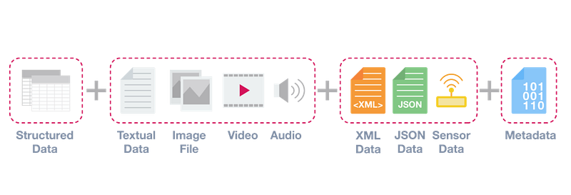
Structured Data
Semi Structured Data
Unstructured Data
Data Warehouse
Data Mart
Data Lake
Pre-requisite to Day 21 is to complete Day 1–20( link below):
Day 3 : Complete Advanced Python for Data Engineering — Part 2
Day 18 : Data Visualization basics, Data Visualization Projects, Data Visualization using Plotly and Bokeh, Data Profiling, Summary Functions, Indexing, Grouping, Linear Regression, Multi Linear Regression, Polynomial Regression, Regression, Support Vector Regression, Decision Tree Regression, Random Forest Regression, Feature Engineering, GroupBy Features, Categorical and Numerical Features, Missing Value Analysis, Fill the missing Values, Unique Value Analysis, Univariate Analysis, Bivariate Analysis, Multivariate Analysis, Correlation Analysis, Spearman’s ρ, Pearson’s r, Kendall’s τ, Cramér’s V (φc), Phik (φk)
Day 20 : ETL ( Extract, Tranform and Load) basics, Why ETL is important?, How ETL works, ETL Tools
Day 21 : Structured Data, Semi Structured Data, Unstructured Data, Data Warehouse, Data Mart, Data Lake
Projects Videos —
All the projects, data structures, SQL, algorithms, system design, Data Science and ML , Data Analytics, Data Engineering, , Implemented Data Science and ML projects, Implemented Data Engineering Projects, Implemented Deep Learning Projects, Implemented Machine Learning Ops Projects, Implemented Time Series Analysis and Forecasting Projects, Implemented Applied Machine Learning Projects, Implemented Tensorflow and Keras Projects, Implemented PyTorch Projects, Implemented Scikit Learn Projects, Implemented Big Data Projects, Implemented Cloud Machine Learning Projects, Implemented Neural Networks Projects, Implemented OpenCV Projects,Complete ML Research Papers Summarized, Implemented Data Analytics projects, Implemented Data Visualization Projects, Implemented Data Mining Projects, Implemented Natural Leaning Processing Projects, MLOps and Deep Learning, Applied Machine Learning with Projects Series, PyTorch with Projects Series, Tensorflow and Keras with Projects Series, Scikit Learn Series with Projects, Time Series Analysis and Forecasting with Projects Series, ML System Design Case Studies Series videos will be published on our youtube channel ( just launched).
Subscribe today!
Tech Newsletter —
If you are interested, you can join my newsletter through which I send tech interview tips, techniques, patterns, hacks — Software Development, ML, Data Science, Startups and Technology projects to more than 30K readers. You can subscribe to Ignito:
System Design Case Studies — In Depth
Design Instagram
Design Netflix
Design Reddit
Design Amazon
Design Messenger App
Design Twitter
Design URL Shortener
Design Dropbox
Design Youtube
Design API Rate Limiter
Design Web Crawler
Design Amazon Prime Video
Design Facebook’s Newsfeed
Design Yelp
Design Uber
Design Tinder
Design Tiktok
Design Whatsapp
Most Popular System Design Questions
Mega Compilation : Solved System Design Case studies
Let’s get started!
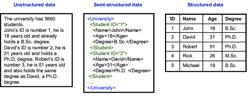
- Structured data refers to data that is organized in a specific format, such as tables in a relational database. It is typically easy to analyze and query because it follows a predefined schema. Examples include data from spreadsheets, tables in a relational database, and data from structured forms.
- Semi-structured data refers to data that has some level of organization, but does not follow a strict schema. It may contain a mix of structured and unstructured elements. Examples include data from JSON, XML, and log files.
- Unstructured data refers to data that does not have a specific format or organization. It is often unorganized and difficult to analyze, but can still provide valuable insights. Examples include data from social media posts, email messages, and images.
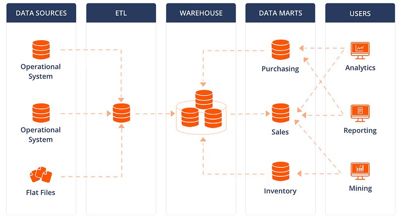
- A Data Warehouse is a large, centralized repository of data that is specifically designed to support business intelligence (BI) activities. It is used to store historical data from various sources, and is optimized for reporting and analysis.
# Connect to the data warehouse
import pyodbc
conn = pyodbc.connect('Driver={SQL Server};Server=localhost;Database=DataWarehouse;Trusted_Connection=yes;')

# Execute SQL queries

# Create a table in the data warehouse
create_table_query = '''
    CREATE TABLE Sales (
        id INT,
        date DATE,
        amount DECIMAL(10,2),
        product VARCHAR(100),
        customer_id INT
    )
'''
cursor = conn.cursor()
cursor.execute(create_table_query)

# Insert data into the data warehouse
insert_data_query = '''
    INSERT INTO Sales (id, date, amount, product, customer_id)
    VALUES (1, '2023-01-01', 100.50, 'Product A', 1),
           (2, '2023-01-02', 200.75, 'Product B', 2),
           (3, '2023-01-03', 150.25, 'Product C', 1)
'''
cursor.execute(insert_data_query)
conn.commit()

# Query data from the data warehouse
select_data_query = 'SELECT * FROM Sales'
cursor.execute(select_data_query)
data = cursor.fetchall()
for row in data:
    print(row)

# Perform aggregations and calculations
aggregate_query = '''
    SELECT product, SUM(amount) AS total_sales
    FROM Sales
    GROUP BY product
'''
cursor.execute(aggregate_query)
result = cursor.fetchall()
for row in result:
    print(row)

# Update data in the data warehouse
update_query = "UPDATE Sales SET amount = amount * 1.1 WHERE product = 'Product A'"
cursor.execute(update_query)
conn.commit()

# Delete data from the data warehouse
delete_query = "DELETE FROM Sales WHERE customer_id = 2"
cursor.execute(delete_query)
conn.commit()

# Close the connection to the data warehouse
conn.close()- A Data Mart is a subset of a data warehouse that is focused on a specific business area, such as sales or finance. It is designed to support the specific reporting and analysis needs of a particular department or business unit.
# Connect to the data mart
import pyodbc
conn = pyodbc.connect('Driver={SQL Server};Server=localhost;Database=DataMart;Trusted_Connection=yes;')

# Execute SQL queries

# Create a table in the data mart
create_table_query = '''
    CREATE TABLE Sales (
        id INT,
        date DATE,
        amount DECIMAL(10,2),
        product VARCHAR(100),
        customer_id INT
    )
'''
cursor = conn.cursor()
cursor.execute(create_table_query)

# Insert data into the data mart
insert_data_query = '''
    INSERT INTO Sales (id, date, amount, product, customer_id)
    VALUES (1, '2023-01-01', 100.50, 'Product A', 1),
           (2, '2023-01-02', 200.75, 'Product B', 2),
           (3, '2023-01-03', 150.25, 'Product C', 1)
'''
cursor.execute(insert_data_query)
conn.commit()

# Query data from the data mart
select_data_query = 'SELECT * FROM Sales'
cursor.execute(select_data_query)
data = cursor.fetchall()
for row in data:
    print(row)

# Perform aggregations and calculations
aggregate_query = '''
    SELECT product, SUM(amount) AS total_sales
    FROM Sales
    GROUP BY product
'''
cursor.execute(aggregate_query)
result = cursor.fetchall()
for row in result:
    print(row)

# Apply filters and conditions
filtered_query = "SELECT * FROM Sales WHERE date >= '2023-01-02'"
cursor.execute(filtered_query)
filtered_data = cursor.fetchall()
for row in filtered_data:
    print(row)

# Close the connection to the data mart
conn.close()- A Data Lake is a large, centralized repository of raw, unstructured data that is stored in its native format. It is designed to store all types of data, structured and unstructured, and is optimized for big data processing and analytics. It allows data scientists to store, process, and analyze data in a single place, and it is often used in conjunction with a data warehouse or data mart.
# Import necessary libraries
from pyspark.sql import SparkSession

# Create a Spark session
spark = SparkSession.builder \
    .appName("DataLakeExample") \
    .config("spark.some.config.option", "some-value") \
    .getOrCreate()

# Read data from a file in the data lake
data = spark.read.format("csv").option("header", "true").load("s3://datalake/input/file.csv")

# Perform transformations and data manipulations
transformed_data = data.select("col1", "col2").filter("col3 > 0").groupBy("col1").sum("col2")

# Write the transformed data back to the data lake
transformed_data.write.format("parquet").mode("overwrite").save("s3://datalake/output/transformed_data.parquet")

# Query data from the data lake
queried_data = spark.sql("SELECT * FROM parquet.`s3://datalake/output/transformed_data.parquet`")

# Perform data analysis and exploration
analysis_result = queried_data.describe()

# Export analysis result to a file in the data lake
analysis_result.write.format("csv").mode("overwrite").save("s3://datalake/output/analysis_result.csv")

# Create external tables for querying data
spark.sql("CREATE EXTERNAL TABLE sales USING parquet LOCATION 's3://datalake/sales_data/'")

# Query data using SQL on the external table
result = spark.sql("SELECT * FROM sales WHERE date >= '2022-01-01'")

# Export the result to a file in the data lake
result.write.format("csv").mode("overwrite").save("s3://datalake/output/query_result.csv")

# Stop the Spark session
spark.stop()
Complete Implementation ( for all)—
# Structured Data

# Read structured data from CSV file
import pandas as pd
data = pd.read_csv('structured_data.csv')

# Perform data analysis and manipulation
data.head()
data.describe()
data.groupby('category').mean()

# Semi-Structured Data

# Read semi-structured data from JSON file
import json
with open('semi_structured_data.json') as f:
    data = json.load(f)

# Access data elements
data['key']
data['nested']['value']

# Unstructured Data

# Read unstructured data from text file
with open('unstructured_data.txt', 'r') as f:
    data = f.read()

# Perform text processing
words = data.split()
unique_words = set(words)
word_counts = {word: words.count(word) for word in unique_words}

# Data Warehouse

# Connect to a data warehouse
import pyodbc
conn = pyodbc.connect('Driver={SQL Server};Server=localhost;Database=DataWarehouse;Trusted_Connection=yes;')

# Execute SQL queries
cursor = conn.cursor()
cursor.execute('SELECT * FROM fact_table')
data = cursor.fetchall()

# Data Mart

# Connect to a data mart
import psycopg2
conn = psycopg2.connect(host="localhost", port="5432", database="DataMart", user="username", password="password")

# Execute SQL queries
cursor = conn.cursor()
cursor.execute('SELECT * FROM dimension_table')
data = cursor.fetchall()

# Data Lake

# Access data in a data lake using Hadoop File System (HDFS)
from pyarrow import hdfs
hdfs_client = hdfs.connect(host='localhost', port=8020)
data = hdfs_client.cat('/data_lake/file.parquet')

# Perform data processing
import pandas as pd
df = pd.read_parquet(data)
df.head()
df.groupby('category').sum()
Snippet —
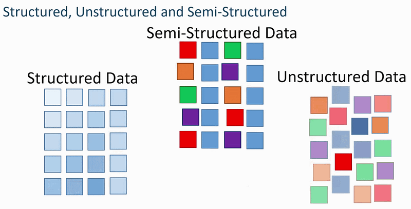
Structured Data
Structured Data is the data which is highly organized, factual and quantitative in nature.
It has a clear data model and can be displayed in rows, columns and relational database.
It consists of numbers, dates, strings and floats and requires less storage.
Advantage of structured data is that it’s easier to manage/maintain and all the legacy data can be stored in a well formatted way.
It resides in the relational databases and data warehouses.
Examples of Structured data —
Numerical data in excel files/google sheets
Ratings on e-commerce website
Relational Databases data
How to deal with Structured Data —
import pandas as pd

# Read structured data from a file (e.g., CSV, Excel)
data = pd.read_csv("data.csv")

# Display the structure and summary of the data
print("Data structure:")
print(data.head())
print("\nData summary:")
print(data.describe())

# Select specific columns
selected_columns = ["column1", "column2", "column3"]
selected_data = data[selected_columns]

# Filter data based on conditions
filtered_data = data[data["column1"] > 10]

# Sort data by a column
sorted_data = data.sort_values("column1")

# Group data and calculate aggregates
grouped_data = data.groupby("column2").agg({"column1": "sum", "column3": "mean"})

# Perform data transformations
transformed_data = data.copy()
transformed_data["new_column"] = transformed_data["column1"] + transformed_data["column2"]

# Perform data analysis
mean_value = data["column1"].mean()
max_value = data["column2"].max()

# Export data to a new file (e.g., CSV, Excel)
transformed_data.to_csv("new_data.csv", index=False)

# Load data from a database
import sqlite3
conn = sqlite3.connect("database.db")
db_data = pd.read_sql_query("SELECT * FROM table", conn)

# Write data to a database table
transformed_data.to_sql("new_table", conn, if_exists="replace")

# Close the database connection
conn.close()
Snippet —
Semi Structured Data
Semi Structured data lacks fixed schema and is loosely organized data which is categorized using meta tags or markers. These are in the form of data files which follow a semi pattern.
Semi structured
Examples of Semi Structured data —
Posts with tags
Tweets with tags
Emails
XML, HTML, JSON Files
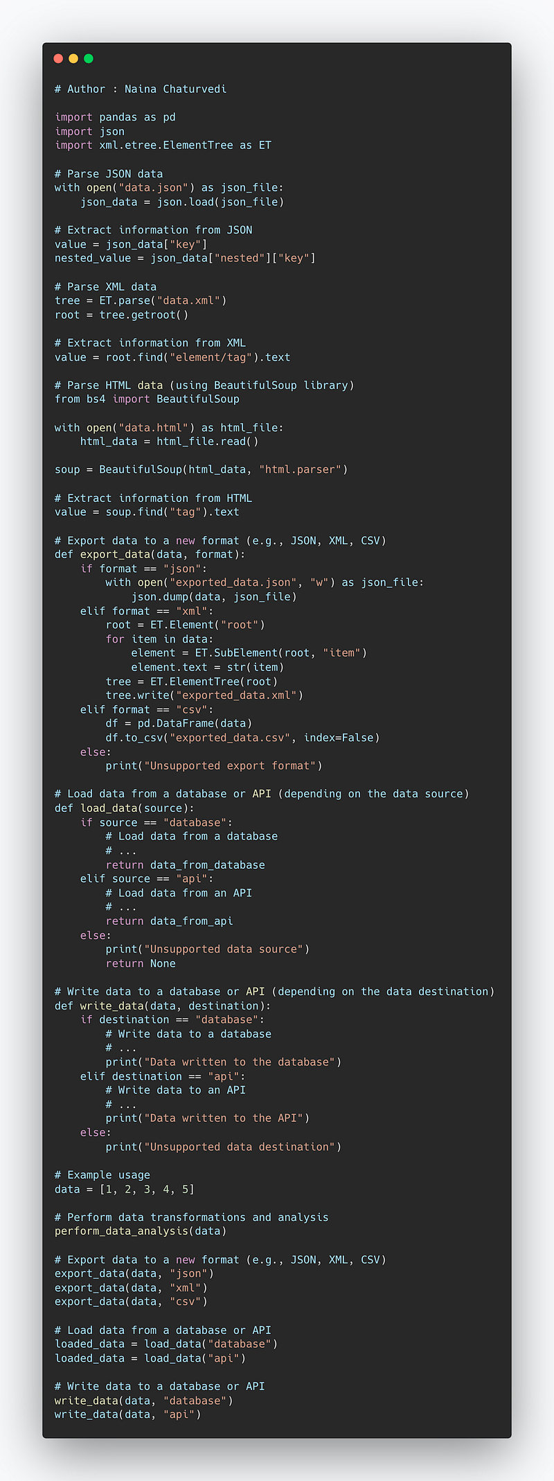
How to deal with Semi-Structured Data —
import pandas as pd
import json
import xml.etree.ElementTree as ET

# Parse JSON data
with open("data.json") as json_file:
    json_data = json.load(json_file)

# Extract information from JSON
value = json_data["key"]
nested_value = json_data["nested"]["key"]

# Parse XML data
tree = ET.parse("data.xml")
root = tree.getroot()

# Extract information from XML
value = root.find("element/tag").text

# Parse HTML data (using BeautifulSoup library)
from bs4 import BeautifulSoup

with open("data.html") as html_file:
    html_data = html_file.read()

soup = BeautifulSoup(html_data, "html.parser")

# Extract information from HTML
value = soup.find("tag").text


# Export data to a new format (e.g., JSON, XML, CSV)
def export_data(data, format):
    if format == "json":
        with open("exported_data.json", "w") as json_file:
            json.dump(data, json_file)
    elif format == "xml":
        root = ET.Element("root")
        for item in data:
            element = ET.SubElement(root, "item")
            element.text = str(item)
        tree = ET.ElementTree(root)
        tree.write("exported_data.xml")
    elif format == "csv":
        df = pd.DataFrame(data)
        df.to_csv("exported_data.csv", index=False)
    else:
        print("Unsupported export format")

# Load data from a database or API (depending on the data source)
def load_data(source):
    if source == "database":
        # Load data from a database
        # ...
        return data_from_database
    elif source == "api":
        # Load data from an API
        # ...
        return data_from_api
    else:
        print("Unsupported data source")
        return None

# Write data to a database or API (depending on the data destination)
def write_data(data, destination):
    if destination == "database":
        # Write data to a database
        # ...
        print("Data written to the database")
    elif destination == "api":
        # Write data to an API
        # ...
        print("Data written to the API")
    else:
        print("Unsupported data destination")

# Example usage
data = [1, 2, 3, 4, 5]

# Perform data transformations and analysis
perform_data_analysis(data)

# Export data to a new format (e.g., JSON, XML, CSV)
export_data(data, "json")
export_data(data, "xml")
export_data(data, "csv")

# Load data from a database or API
loaded_data = load_data("database")
loaded_data = load_data("api")

# Write data to a database or API
write_data(data, "database")
write_data(data, "api")
Snippet —
Unstructured Data
Unstructured data doesn’t have an inherent structure and stores in different types of formats and files. It doesn’t have predefined data models and very difficult to search the data. It’s qualitative in nature and the schema creation of read.
It cannot be displayed in rows, columns or relational database formats. It requires more storage and more difficult to manage as well as maintain.
It resides on NOSQL Databases and Data lakes and Data warehouses.
Examples of Unstructured Data —
Surveys, transcripts
pdfs, images, videos etc
Emails
Audio Files
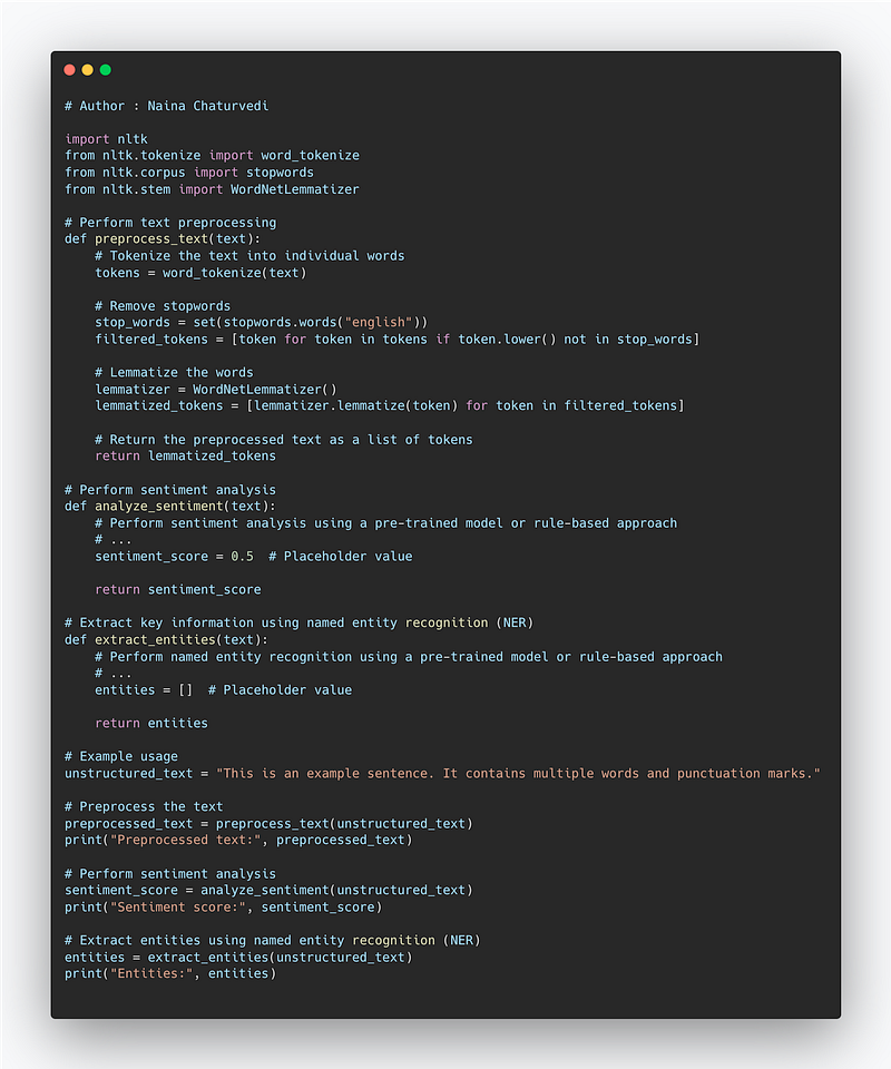
How to handle Unstructured Data —
import nltk
from nltk.tokenize import word_tokenize
from nltk.corpus import stopwords
from nltk.stem import WordNetLemmatizer

# Perform text preprocessing
def preprocess_text(text):
    # Tokenize the text into individual words
    tokens = word_tokenize(text)

    # Remove stopwords
    stop_words = set(stopwords.words("english"))
    filtered_tokens = [token for token in tokens if token.lower() not in stop_words]

    # Lemmatize the words
    lemmatizer = WordNetLemmatizer()
    lemmatized_tokens = [lemmatizer.lemmatize(token) for token in filtered_tokens]

    # Return the preprocessed text as a list of tokens
    return lemmatized_tokens

# Perform sentiment analysis
def analyze_sentiment(text):
    # Perform sentiment analysis using a pre-trained model or rule-based approach
    # ...
    sentiment_score = 0.5  # Placeholder value

    return sentiment_score

# Extract key information using named entity recognition (NER)
def extract_entities(text):
    # Perform named entity recognition using a pre-trained model or rule-based approach
    # ...
    entities = []  # Placeholder value

    return entities

# Example usage
unstructured_text = "This is an example sentence. It contains multiple words and punctuation marks."

# Preprocess the text
preprocessed_text = preprocess_text(unstructured_text)
print("Preprocessed text:", preprocessed_text)

# Perform sentiment analysis
sentiment_score = analyze_sentiment(unstructured_text)
print("Sentiment score:", sentiment_score)

# Extract entities using named entity recognition (NER)
entities = extract_entities(unstructured_text)
print("Entities:", entities)
Snippet —
Data Warehousing
It summarizes the data and stores historical and up to date present information from various data sources. The data is structured and processed, non volatile and time variant.
It’s very expensive for large data volumes and is less agile with fixed configuration.
Data Mart
Data Mart is the condensed summarized data which is like focussed data from different organizations/departments. It’s highly focussed and requires high level of prior processing.
Data Lake
Data lake contains the data which is raw, structured/semi-structured/unstructured. It’s designed for the low cost storage and is highly agile that you can configure as and when required. It’s used by the data scientists in its native format that makes it very flexible to use to analyze and build models from various data systems/sources.
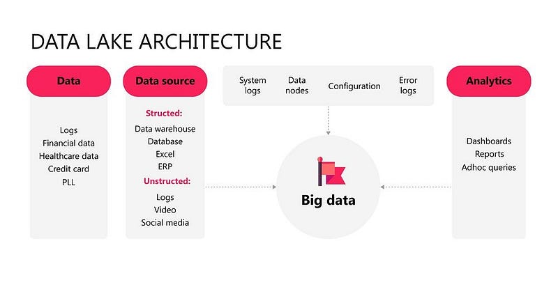
It’s used for machine learning, discovery and deep analysis.
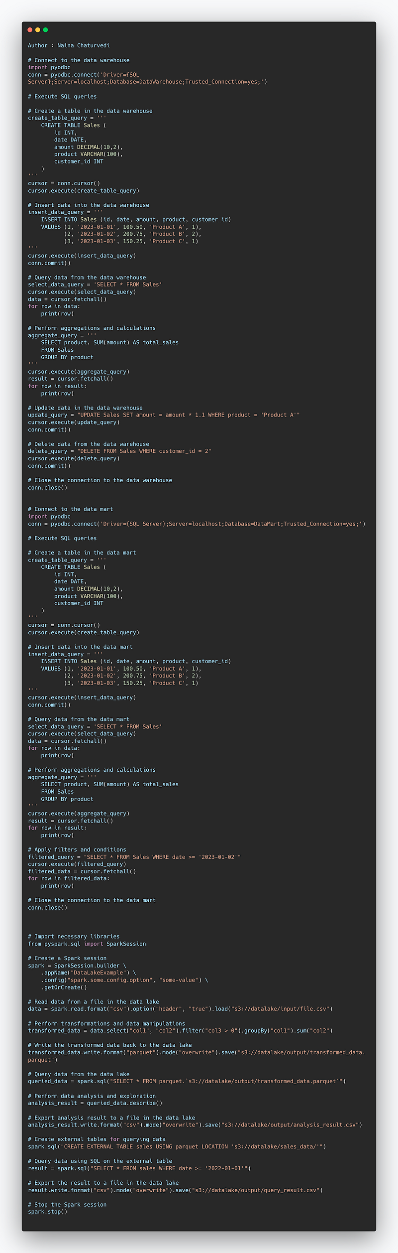
Complete Code — Data Warehouse, Data Mart and Data Lake:
Author : Naina Chaturvedi

# Connect to the data warehouse
import pyodbc
conn = pyodbc.connect('Driver={SQL Server};Server=localhost;Database=DataWarehouse;Trusted_Connection=yes;')

# Execute SQL queries

# Create a table in the data warehouse
create_table_query = '''
    CREATE TABLE Sales (
        id INT,
        date DATE,
        amount DECIMAL(10,2),
        product VARCHAR(100),
        customer_id INT
    )
'''
cursor = conn.cursor()
cursor.execute(create_table_query)

# Insert data into the data warehouse
insert_data_query = '''
    INSERT INTO Sales (id, date, amount, product, customer_id)
    VALUES (1, '2023-01-01', 100.50, 'Product A', 1),
           (2, '2023-01-02', 200.75, 'Product B', 2),
           (3, '2023-01-03', 150.25, 'Product C', 1)
'''
cursor.execute(insert_data_query)
conn.commit()

# Query data from the data warehouse
select_data_query = 'SELECT * FROM Sales'
cursor.execute(select_data_query)
data = cursor.fetchall()
for row in data:
    print(row)

# Perform aggregations and calculations
aggregate_query = '''
    SELECT product, SUM(amount) AS total_sales
    FROM Sales
    GROUP BY product
'''
cursor.execute(aggregate_query)
result = cursor.fetchall()
for row in result:
    print(row)

# Update data in the data warehouse
update_query = "UPDATE Sales SET amount = amount * 1.1 WHERE product = 'Product A'"
cursor.execute(update_query)
conn.commit()

# Delete data from the data warehouse
delete_query = "DELETE FROM Sales WHERE customer_id = 2"
cursor.execute(delete_query)
conn.commit()

# Close the connection to the data warehouse
conn.close()


# Connect to the data mart
import pyodbc
conn = pyodbc.connect('Driver={SQL Server};Server=localhost;Database=DataMart;Trusted_Connection=yes;')

# Execute SQL queries

# Create a table in the data mart
create_table_query = '''
    CREATE TABLE Sales (
        id INT,
        date DATE,
        amount DECIMAL(10,2),
        product VARCHAR(100),
        customer_id INT
    )
'''
cursor = conn.cursor()
cursor.execute(create_table_query)

# Insert data into the data mart
insert_data_query = '''
    INSERT INTO Sales (id, date, amount, product, customer_id)
    VALUES (1, '2023-01-01', 100.50, 'Product A', 1),
           (2, '2023-01-02', 200.75, 'Product B', 2),
           (3, '2023-01-03', 150.25, 'Product C', 1)
'''
cursor.execute(insert_data_query)
conn.commit()

# Query data from the data mart
select_data_query = 'SELECT * FROM Sales'
cursor.execute(select_data_query)
data = cursor.fetchall()
for row in data:
    print(row)

# Perform aggregations and calculations
aggregate_query = '''
    SELECT product, SUM(amount) AS total_sales
    FROM Sales
    GROUP BY product
'''
cursor.execute(aggregate_query)
result = cursor.fetchall()
for row in result:
    print(row)

# Apply filters and conditions
filtered_query = "SELECT * FROM Sales WHERE date >= '2023-01-02'"
cursor.execute(filtered_query)
filtered_data = cursor.fetchall()
for row in filtered_data:
    print(row)

# Close the connection to the data mart
conn.close()


# Import necessary libraries
from pyspark.sql import SparkSession

# Create a Spark session
spark = SparkSession.builder \
    .appName("DataLakeExample") \
    .config("spark.some.config.option", "some-value") \
    .getOrCreate()

# Read data from a file in the data lake
data = spark.read.format("csv").option("header", "true").load("s3://datalake/input/file.csv")

# Perform transformations and data manipulations
transformed_data = data.select("col1", "col2").filter("col3 > 0").groupBy("col1").sum("col2")

# Write the transformed data back to the data lake
transformed_data.write.format("parquet").mode("overwrite").save("s3://datalake/output/transformed_data.parquet")

# Query data from the data lake
queried_data = spark.sql("SELECT * FROM parquet.`s3://datalake/output/transformed_data.parquet`")

# Perform data analysis and exploration
analysis_result = queried_data.describe()

# Export analysis result to a file in the data lake
analysis_result.write.format("csv").mode("overwrite").save("s3://datalake/output/analysis_result.csv")

# Create external tables for querying data
spark.sql("CREATE EXTERNAL TABLE sales USING parquet LOCATION 's3://datalake/sales_data/'")

# Query data using SQL on the external table
result = spark.sql("SELECT * FROM sales WHERE date >= '2022-01-01'")

# Export the result to a file in the data lake
result.write.format("csv").mode("overwrite").save("s3://datalake/output/query_result.csv")

# Stop the Spark session
spark.stop()
Snippet —
That’s it for now.
Find Day 22 Below:
Let me know if you have questions in the comment section below. Subscribe/ Follow, Like/Clap as it would encourage me to write more in my free time
Stay Tuned!!
Read more —
All the Complete System Design Series Parts —
6. Networking, How Browsers work, Content Network Delivery ( CDN)
Github —
For Python Projects —
For complete 60 days of Data Science and ML : Day 1 — Day 60 : Quick Recap of 60 days of Data Science and ML
Follow for more updates. Stay tuned and keep coding!
For other projects, tune to —
Build Machine Learning Pipelines( With Code)
Recurrent Neural Network with Keras
Clustering Geolocation Data in Python using DBSCAN and K-Means
Facial Expression Recognition using Keras
Hyperparameter Tuning with Keras Tuner
Custom Layers in Keras


