Day 15 of 30 days of Data Engineering Series with Projects

Welcome back peeps to Day 15 of Data Engineering Series with Projects!

In this we will cover —

Advanced Pandas Techniques

Split data using pandas

Binning Data

Mean Imputation and Interpolate method

Combining Data using Concat and Join

Pre-requisite to Day 15 is to complete Day 1–14( link below):

Day 1 : What’s Data Engineering, Why Data Engineering, Data Engineers — ML Engineers — Data Scientists, Purpose and Scope

Day 2 : Complete Python for Data Engineering — Part 1

Day 3 : Complete Advanced Python for Data Engineering — Part 2

Day 4: Techniques to write efficient and Optimized Code

Day 5 : SQL

Day 6 : Advanced SQL

Day 7 : BigQuery and SQL vs NOSQL databases

Day 8 : Advanced Functions

Day 9 : Query Optimizations

Day 10 : MySQL and PostgreSQL

Day 11: Shell scripting and Linux “touch” command

Day 12 : Map Reduce, Data Warehouse, Data Lakes

Day 13: Pandas, Pandas, Data Cleaning and processing, Outlier Detection, Noisy Data, Missing Data, Pandas Functions, Aggregate Functions, Joins

Day 14 : Numpy

Day 15 : Advanced Pandas Techniques

Projects Videos —

Subscribe today!

Ignito

Excited to share that we have launched our Youtube channel — Ignito to cover all the projects and coding exercise for …

www.youtube.com

Tech Newsletter —

If you are interested, you can join my newsletter through which I send tech interview tips, techniques, patterns, hacks — Software Development, ML, Data Science, Startups and Technology projects to more than 30K readers. You can subscribe to Ignito:

Ignito

Data Science, ML, AI and more… Click to read Ignito, by Naina Chaturvedi, a Substack publication with hundreds of…

naina0405.substack.com

System Design Case Studies — In Depth

Design Instagram

Design Netflix

Design Reddit

Design Amazon

Design Messenger App

Design Twitter

Design URL Shortener

Design Dropbox

Design Youtube

Design API Rate Limiter

Design Web Crawler

Design Amazon Prime Video

Design Facebook’s Newsfeed

Design Yelp

Design Uber

Design Tinder

Design Tiktok

Design Whatsapp

Mega Compilation : Solved System Design Case studies

This is Day 15 of 30 days of Data Engineering Series where we will be covering —

Advanced Pandas Techniques

Let’s get started!

Real world data is messy ( it contains null values, noises, missing values etc) and in most of the cases when we start the building the ML model we need to clean, format and pre process the data.

Splitting data using pandas can be done using the train_test_split function from the sklearn.model_selection module. This function allows you to split a dataset into training and testing sets.
Binning data involves grouping a set of continuous or numerical data into a smaller number of discrete “bins” or ranges. This can be done using the cut or qcut functions in pandas, which allow you to specify the number of bins and the labels for each bin.
Mean imputation is a method of replacing missing values with the mean value of the dataset. This can be done using the fillna function in pandas and passing in the mean value of the dataset.
Interpolation is a method of estimating missing values by taking the average of the values on either side of the missing data point. This can be done using the interpolate function in pandas, which can use various interpolation methods such as linear or polynomial.
Combining data using pandas can be done using the concat function to concatenate multiple dataframes along a particular axis, or the join function to join two dataframes on a common column or index.

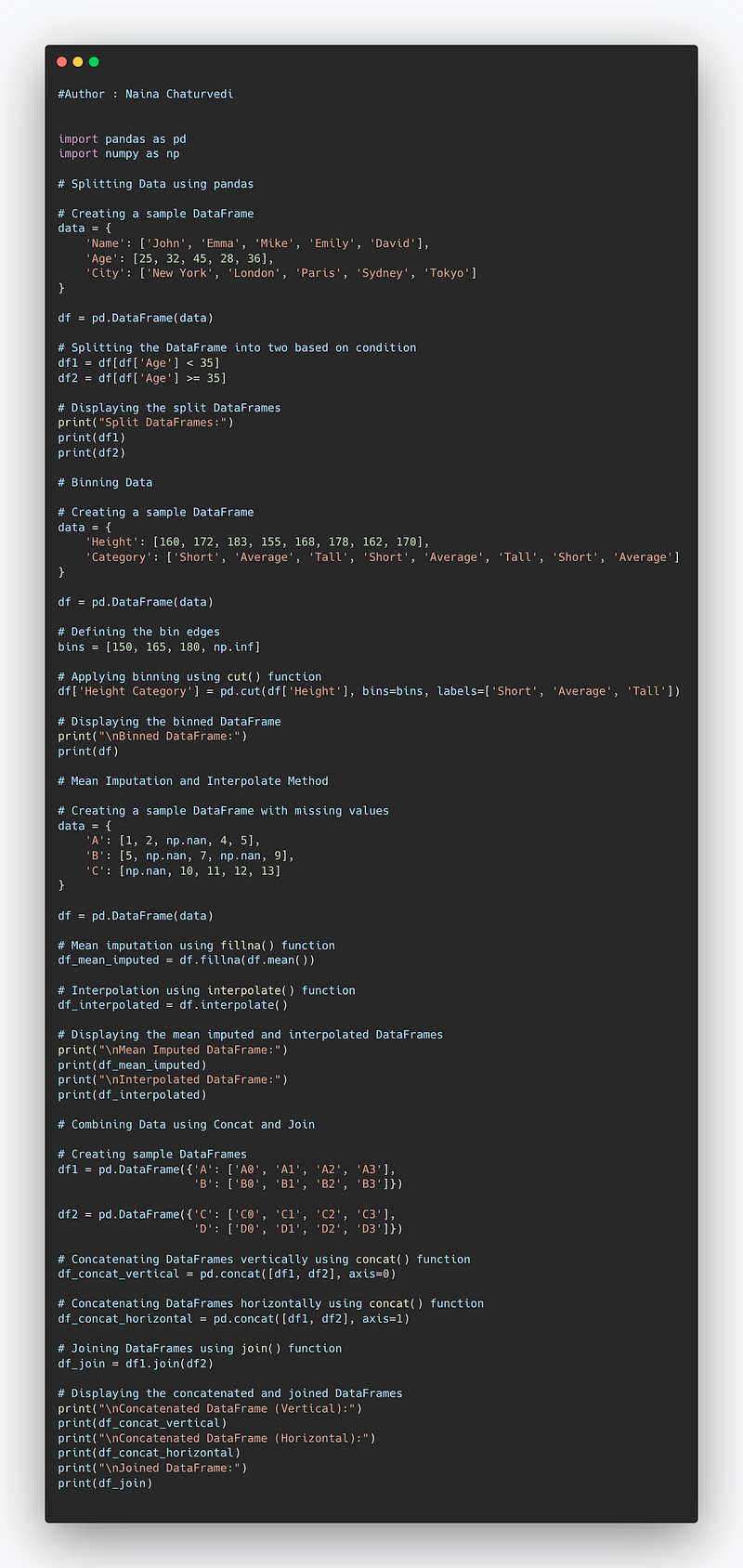
Code Implementation —

import pandas as pd
import numpy as np

# Splitting Data using pandas

# Creating a sample DataFrame
data = {
    'Name': ['John', 'Emma', 'Mike', 'Emily', 'David'],
    'Age': [25, 32, 45, 28, 36],
    'City': ['New York', 'London', 'Paris', 'Sydney', 'Tokyo']
}

df = pd.DataFrame(data)

# Splitting the DataFrame into two based on condition
df1 = df[df['Age'] < 35]
df2 = df[df['Age'] >= 35]

# Displaying the split DataFrames
print("Split DataFrames:")
print(df1)
print(df2)

# Binning Data

# Creating a sample DataFrame
data = {
    'Height': [160, 172, 183, 155, 168, 178, 162, 170],
    'Category': ['Short', 'Average', 'Tall', 'Short', 'Average', 'Tall', 'Short', 'Average']
}

df = pd.DataFrame(data)

# Defining the bin edges
bins = [150, 165, 180, np.inf]

# Applying binning using cut() function
df['Height Category'] = pd.cut(df['Height'], bins=bins, labels=['Short', 'Average', 'Tall'])

# Displaying the binned DataFrame
print("\nBinned DataFrame:")
print(df)

# Mean Imputation and Interpolate Method

# Creating a sample DataFrame with missing values
data = {
    'A': [1, 2, np.nan, 4, 5],
    'B': [5, np.nan, 7, np.nan, 9],
    'C': [np.nan, 10, 11, 12, 13]
}

df = pd.DataFrame(data)

# Mean imputation using fillna() function
df_mean_imputed = df.fillna(df.mean())

# Interpolation using interpolate() function
df_interpolated = df.interpolate()

# Displaying the mean imputed and interpolated DataFrames
print("\nMean Imputed DataFrame:")
print(df_mean_imputed)
print("\nInterpolated DataFrame:")
print(df_interpolated)

# Combining Data using Concat and Join

# Creating sample DataFrames
df1 = pd.DataFrame({'A': ['A0', 'A1', 'A2', 'A3'],
                    'B': ['B0', 'B1', 'B2', 'B3']})

df2 = pd.DataFrame({'C': ['C0', 'C1', 'C2', 'C3'],
                    'D': ['D0', 'D1', 'D2', 'D3']})

# Concatenating DataFrames vertically using concat() function
df_concat_vertical = pd.concat([df1, df2], axis=0)

# Concatenating DataFrames horizontally using concat() function
df_concat_horizontal = pd.concat([df1, df2], axis=1)

# Joining DataFrames using join() function
df_join = df1.join(df2)

# Displaying the concatenated and joined DataFrames
print("\nConcatenated DataFrame (Vertical):")
print(df_concat_vertical)
print("\nConcatenated DataFrame (Horizontal):")
print(df_concat_horizontal)
print("\nJoined DataFrame:")
print(df_join)

Snippet —

Before you start implementing these techniques, load the data of your choice in your working environment. For this post, I’m using Iris data.

Start with importing the necessary libraries such as Pandas and Numpy and loading your data set. Once done, dive in the techniques below —

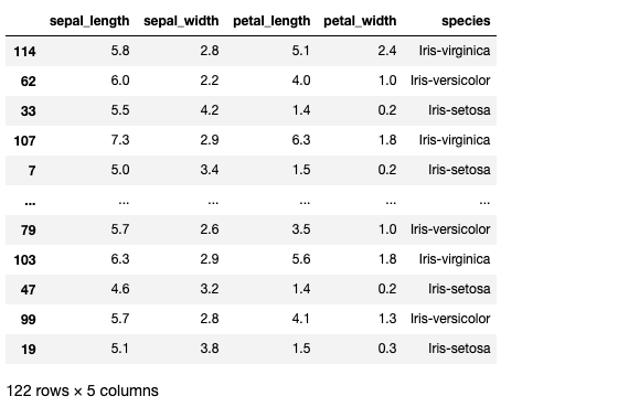
1. Split data using pandas

In the code below, we are splitting the data into a random sample of rows and removing them from the original data after dropping index values.

iris_data_new= df.copy()
df1=iris_data_new.sample(frac=0.75,random_state=0)
iris_data_new=iris_data_new.drop(df1.index)

df2=iris_data_new.sample(frac=0.25,random_state=0)
iris_data_new=iris_data_new.drop(df2.index)

print(df1.shape)

Output —

(112, 5)

2. Binning Data

Binning is a technique to group/bin your data into multiple buckets which is very helpful if you dealing with continuous numeric data. In pandas you can bin the data using functions cut and cut. First check the shape of your data i.e no of rows and columns.

print(iris_data.shape)

Output —

(150, 5)

Then bin your data using qcut as shown below —

pd.qcut(df['sepal_width'],q=5).value_counts()

Output —

(2.7, 3.0]      50
(1.999, 2.7]    33
(3.1, 3.4]      31
(3.4, 4.4]      24
(3.0, 3.1]      12
Name: sepal_width, dtype: int64

3. Slicing using loc and iloc functions

You can do position based and label based slicing using iloc and loc functions respectively.

iris_data.loc[100:105, 'petal_length':'species']

Output —

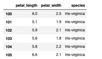
iris_data.iloc[:4]

Output —

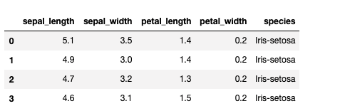
4. Mean Imputation and Interpolate method

Mean Imputation is a technique in which the missing value is replaced by the mean of available data in the chosen column.

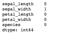
First see if your data has missing values or not.

iris_data.isnull().sum()

Output —

Then calculate the mean and replace the missing value —

iris_data['sepal_width'].mean()

Output —

3.0516778523489942

Replace the missing value

iris_data['sepal_width'].fillna(iris_data['sepal_width'].mean(), inplace=True)
iris_data.isnull().sum()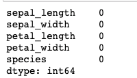

Interpolate method —

iris_data['sepal_width'].fillna(iris_data['sepal_width'].interpolate(), inplace=True)

5. Combining Data using Concat and Join

Just like in numpy, pd.concat() function is used for concatenation of Series or DataFrame objects in pandas.

df4=pd.concat([df1,df2],axis=0)

print(df4)

Output —

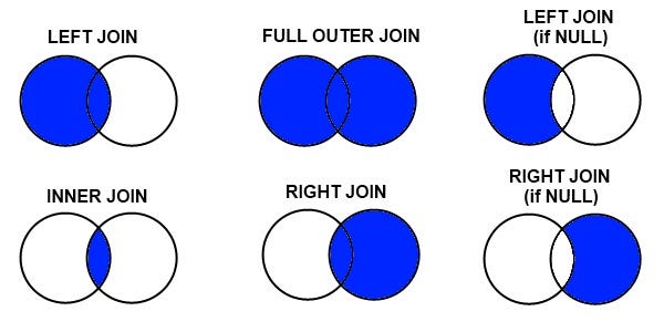
Joins —

Merging and joining the data is one of the most important skill in the data science. Understanding and Implementing it right is crucial in order to analyze data well.

In this we will implement —

Inner Join : keep rows from both the tables/data frames based on the specified merge condition.
Full Join : keep all the rows form left table and right table with matched rows wherever possible and NaN’s elsewhere.
Left Join : keep all the rows form left table and wherever there are missing values in the right table, put it as NaN’s, based on the specified merge condition.
Right Join : keep all the rows form right table and wherever there are missing values in the left table, put it as NaN’s, based on the specified merge condition.

#Inner Join
df5=pd.merge(df1,df2,on='sepal_length')
print(df5)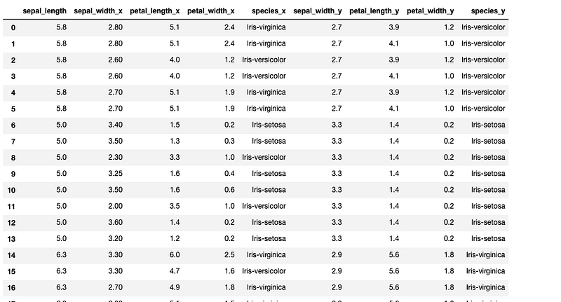

#Full outer join
df6=pd.merge(df1,df2,how='outer')
print(df6)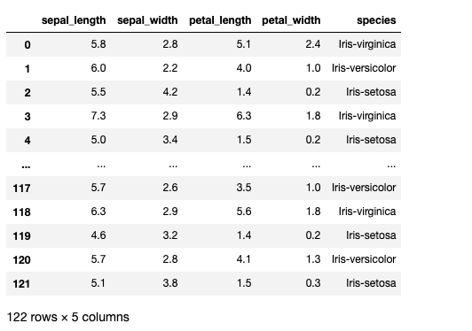

#Left Join
df7=pd.merge(df1,df2,how='left')
print(df7)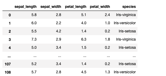

#Right Join
df8=pd.merge(df1,df2,how='right')
print(df8)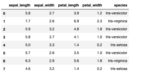

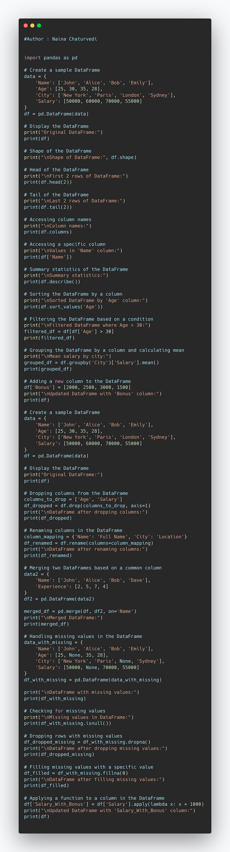
Complete Code —

import pandas as pd

# Create a sample DataFrame
data = {
    'Name': ['John', 'Alice', 'Bob', 'Emily'],
    'Age': [25, 30, 35, 28],
    'City': ['New York', 'Paris', 'London', 'Sydney'],
    'Salary': [50000, 60000, 70000, 55000]
}
df = pd.DataFrame(data)

# Display the DataFrame
print("Original DataFrame:")
print(df)

# Shape of the DataFrame
print("\nShape of DataFrame:", df.shape)

# Head of the DataFrame
print("\nFirst 2 rows of DataFrame:")
print(df.head(2))

# Tail of the DataFrame
print("\nLast 2 rows of DataFrame:")
print(df.tail(2))

# Accessing column names
print("\nColumn names:")
print(df.columns)

# Accessing a specific column
print("\nValues in 'Name' column:")
print(df['Name'])

# Summary statistics of the DataFrame
print("\nSummary statistics:")
print(df.describe())

# Sorting the DataFrame by a column
print("\nSorted DataFrame by 'Age' column:")
print(df.sort_values('Age'))

# Filtering the DataFrame based on a condition
print("\nFiltered DataFrame where Age > 30:")
filtered_df = df[df['Age'] > 30]
print(filtered_df)

# Grouping the DataFrame by a column and calculating mean
print("\nMean salary by city:")
grouped_df = df.groupby('City')['Salary'].mean()
print(grouped_df)

# Adding a new column to the DataFrame
df['Bonus'] = [2000, 2500, 3000, 1500]
print("\nUpdated DataFrame with 'Bonus' column:")
print(df)


# Create a sample DataFrame
data = {
    'Name': ['John', 'Alice', 'Bob', 'Emily'],
    'Age': [25, 30, 35, 28],
    'City': ['New York', 'Paris', 'London', 'Sydney'],
    'Salary': [50000, 60000, 70000, 55000]
}
df = pd.DataFrame(data)

# Display the DataFrame
print("Original DataFrame:")
print(df)

# Dropping columns from the DataFrame
columns_to_drop = ['Age', 'Salary']
df_dropped = df.drop(columns_to_drop, axis=1)
print("\nDataFrame after dropping columns:")
print(df_dropped)

# Renaming columns in the DataFrame
column_mapping = {'Name': 'Full Name', 'City': 'Location'}
df_renamed = df.rename(columns=column_mapping)
print("\nDataFrame after renaming columns:")
print(df_renamed)

# Merging two DataFrames based on a common column
data2 = {
    'Name': ['John', 'Alice', 'Bob', 'Dave'],
    'Experience': [2, 5, 7, 4]
}
df2 = pd.DataFrame(data2)

merged_df = pd.merge(df, df2, on='Name')
print("\nMerged DataFrame:")
print(merged_df)

# Handling missing values in the DataFrame
data_with_missing = {
    'Name': ['John', 'Alice', 'Bob', 'Emily'],
    'Age': [25, None, 35, 28],
    'City': ['New York', 'Paris', None, 'Sydney'],
    'Salary': [50000, None, 70000, 55000]
}
df_with_missing = pd.DataFrame(data_with_missing)

print("\nDataFrame with missing values:")
print(df_with_missing)

# Checking for missing values
print("\nMissing values in DataFrame:")
print(df_with_missing.isnull())

# Dropping rows with missing values
df_dropped_missing = df_with_missing.dropna()
print("\nDataFrame after dropping missing values:")
print(df_dropped_missing)

# Filling missing values with a specific value
df_filled = df_with_missing.fillna(0)
print("\nDataFrame after filling missing values:")
print(df_filled)

# Applying a function to a column in the DataFrame
df['Salary_With_Bonus'] = df['Salary'].apply(lambda x: x + 1000)
print("\nUpdated DataFrame with 'Salary_With_Bonus' column:")
print(df)

Snippet —

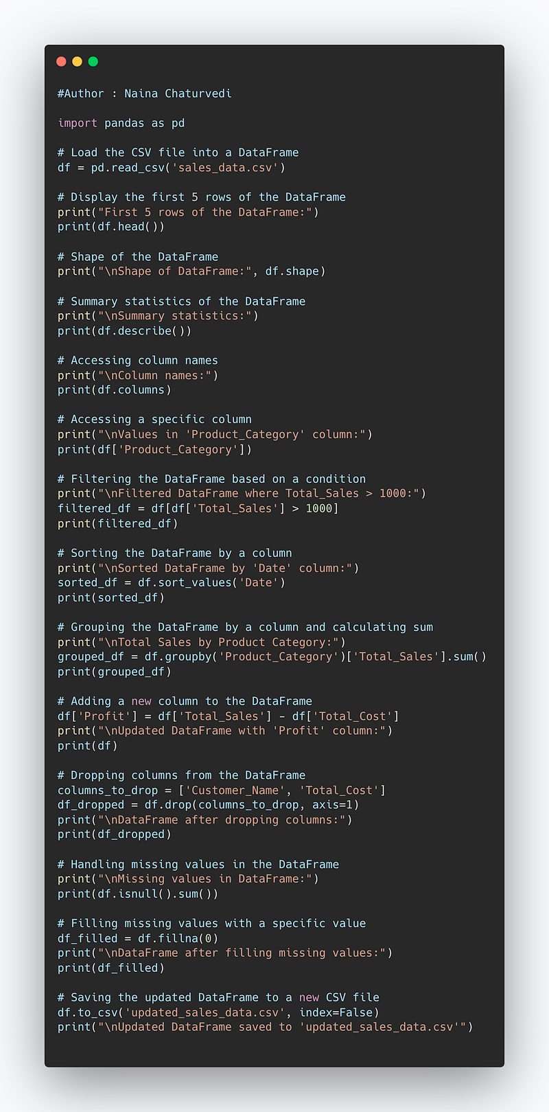
Code Implementation —

import pandas as pd

# Load the CSV file into a DataFrame
df = pd.read_csv('sales_data.csv')

# Display the first 5 rows of the DataFrame
print("First 5 rows of the DataFrame:")
print(df.head())

# Shape of the DataFrame
print("\nShape of DataFrame:", df.shape)

# Summary statistics of the DataFrame
print("\nSummary statistics:")
print(df.describe())

# Accessing column names
print("\nColumn names:")
print(df.columns)

# Accessing a specific column
print("\nValues in 'Product_Category' column:")
print(df['Product_Category'])

# Filtering the DataFrame based on a condition
print("\nFiltered DataFrame where Total_Sales > 1000:")
filtered_df = df[df['Total_Sales'] > 1000]
print(filtered_df)

# Sorting the DataFrame by a column
print("\nSorted DataFrame by 'Date' column:")
sorted_df = df.sort_values('Date')
print(sorted_df)

# Grouping the DataFrame by a column and calculating sum
print("\nTotal Sales by Product Category:")
grouped_df = df.groupby('Product_Category')['Total_Sales'].sum()
print(grouped_df)

# Adding a new column to the DataFrame
df['Profit'] = df['Total_Sales'] - df['Total_Cost']
print("\nUpdated DataFrame with 'Profit' column:")
print(df)

# Dropping columns from the DataFrame
columns_to_drop = ['Customer_Name', 'Total_Cost']
df_dropped = df.drop(columns_to_drop, axis=1)
print("\nDataFrame after dropping columns:")
print(df_dropped)

# Handling missing values in the DataFrame
print("\nMissing values in DataFrame:")
print(df.isnull().sum())

# Filling missing values with a specific value
df_filled = df.fillna(0)
print("\nDataFrame after filling missing values:")
print(df_filled)

# Saving the updated DataFrame to a new CSV file
df.to_csv('updated_sales_data.csv', index=False)
print("\nUpdated DataFrame saved to 'updated_sales_data.csv'")

Snippet —

That’s it for now.

Find Day 16 Below —

Day 16 of 30 days of Data Engineering Series with Projects

Welcome back peeps to Day 16 of Data Engineering Series with Projects!

medium.com

Let me know if you have questions in the comment section below. Subscribe/ Follow, Like/Clap as it would encourage me to write more in my free time

Stay Tuned!!

All the Complete System Design Series Parts —

1. System design basics

2. Horizontal and vertical scaling

3. Load balancing and Message queues

4. High level design and low level design, Consistent Hashing, Monolithic and Microservices architecture

5. Caching, Indexing, Proxies

6. Networking, How Browsers work, Content Network Delivery ( CDN)

7. Database Sharding, CAP Theorem, Database schema Design

8. Concurrency, API, Components + OOP + Abstraction

9. Estimation and Planning, Performance

10. Map Reduce, Patterns and Microservices

11. SQL vs NoSQL and Cloud

12. Most Popular System Design Questions

Github —

Complete-System-Design/README.md at main · Coder-World04/Complete-System-Design

This repository contains everything you need to become proficient in System Design Topics you should know in System…

github.com

Keep learning and coding ;)

Day 5 coming soon!

For Python Projects —

Complete Python And Projects — Mega Compilation

Everything that you need to know in Python with Projects…

medium.com

Analyzing Video using Python, OpenCV and NumPy

With Code Implementation…

medium.datadriveninvestor.com

For complete 60 days of Data Science and ML : Day 1 — Day 60 : Quick Recap of 60 days of Data Science and ML

Day 1 — Day 60 : Quick Recap of 60 days of Data Science and ML

Connect the ML dots…

medium.com

Follow for more updates. Stay tuned and keep coding! Disclosure: Some of the links are affiliates.

For other projects, tune to —

Build Machine Learning Pipelines( With Code)

Build Machine Learning Pipelines( With Code) — Part 1

Complete implementation…

medium.datadriveninvestor.com

Recurrent Neural Network with Keras

Recurrent Neural Network with Keras

Project Implementation and cheatsheet…

medium.datadriveninvestor.com

Clustering Geolocation Data in Python using DBSCAN and K-Means

Clustering Geolocation Data in Python using DBSCAN and K-Means

Project Implementation…

medium.datadriveninvestor.com

Facial Expression Recognition using Keras

Facial Expression Recognition using Keras

Project Implementation…

medium.datadriveninvestor.com

Hyperparameter Tuning with Keras Tuner

Hyperparameter Tuning with Keras Tuner

Project Implementation….

medium.datadriveninvestor.com

Custom Layers in Keras

Custom Layers in Keras

Code implementation …

medium.datadriveninvestor.com

Day 15 of 30 days of Data Engineering Series with Projects

Advanced Pandas Techniques

Ignito

Excited to share that we have launched our Youtube channel — Ignito to cover all the projects and coding exercise for …

Tech Newsletter —

Ignito

Data Science, ML, AI and more… Click to read Ignito, by Naina Chaturvedi, a Substack publication with hundreds of…

System Design Case Studies — In Depth

Design Instagram

Design Netflix

Design Reddit

Design Amazon

Design Messenger App

Design Twitter

Design URL Shortener

Design Dropbox

Design Youtube

Design API Rate Limiter

Design Web Crawler

Design Amazon Prime Video

Design Facebook’s Newsfeed

Design Yelp

Design Uber

Design Tinder

Design Tiktok

Design Whatsapp

Most Popular System Design Questions

Mega Compilation : Solved System Design Case studies

Advanced Pandas Techniques

1. Split data using pandas

2. Binning Data

3. Slicing using loc and iloc functions

4. Mean Imputation and Interpolate method

5. Combining Data using Concat and Join

Joins —

That’s it for now.

Find Day 16 Below —

Day 16 of 30 days of Data Engineering Series with Projects

Welcome back peeps to Day 16 of Data Engineering Series with Projects!

Read more —

All the Complete System Design Series Parts —

Github —

Complete-System-Design/README.md at main · Coder-World04/Complete-System-Design

This repository contains everything you need to become proficient in System Design Topics you should know in System…

For Python Projects —

Complete Python And Projects — Mega Compilation

Everything that you need to know in Python with Projects…

Analyzing Video using Python, OpenCV and NumPy

With Code Implementation…

Day 1 — Day 60 : Quick Recap of 60 days of Data Science and ML

Connect the ML dots…

For other projects, tune to —

Build Machine Learning Pipelines( With Code) — Part 1

Complete implementation…

Recurrent Neural Network with Keras

Project Implementation and cheatsheet…

Clustering Geolocation Data in Python using DBSCAN and K-Means

Project Implementation…

Facial Expression Recognition using Keras

Project Implementation…

Hyperparameter Tuning with Keras Tuner

Project Implementation….

Custom Layers in Keras

Code implementation …