Day 16 of 30 days of Data Engineering Series with Projects

Welcome back peeps to Day 16 of Data Engineering Series with Projects!

In this we will cover —

Data Pre-processing

Handling missing values

Data Cleaning

Mean/mode/median Imputation

Hot Deck Imputation

Rescale Data

Binarize Data

Regression Imputation

Stochastic regression imputation

Feature Scaling

Pre-requisite to Day 16 is to complete Day 1–15( link below):

Day 1 : What’s Data Engineering, Why Data Engineering, Data Engineers — ML Engineers — Data Scientists, Purpose and Scope

Day 2 : Complete Python for Data Engineering — Part 1

Day 3 : Complete Advanced Python for Data Engineering — Part 2

Day 4: Techniques to write efficient and Optimized Code

Day 5 : SQL

Day 6 : Advanced SQL

Day 7 : BigQuery and SQL vs NOSQL databases

Day 8 : Advanced Functions

Day 9 : Query Optimizations

Day 10 : MySQL and PostgreSQL

Day 11: Shell scripting and Linux “touch” command

Day 12 : Map Reduce, Data Warehouse, Data Lakes

Day 13: Pandas, Pandas, Data Cleaning and processing, Outlier Detection, Noisy Data, Missing Data, Pandas Functions, Aggregate Functions, Joins

Day 14 : Numpy

Day 15 : Advanced Pandas Techniques

Day 16 : Data Pre-processing, Handling missing values, Data Cleaning, Mean/mode/median Imputation, Hot Deck Imputation, Rescale Data, Binarize Data, Regression Imputation, Stochastic regression imputation, Feature Scaling

Projects Videos —

All the projects, data structures, SQL, algorithms, system design, Data Science and ML , Data Analytics, Data Engineering, , Implemented Data Science and ML projects, Implemented Data Engineering Projects, Implemented Deep Learning Projects, Implemented Machine Learning Ops Projects, Implemented Time Series Analysis and Forecasting Projects, Implemented Applied Machine Learning Projects, Implemented Tensorflow and Keras Projects, Implemented PyTorch Projects, Implemented Scikit Learn Projects, Implemented Big Data Projects, Implemented Cloud Machine Learning Projects, Implemented Neural Networks Projects, Implemented OpenCV Projects,Complete ML Research Papers Summarized, Implemented Data Analytics projects, Implemented Data Visualization Projects, Implemented Data Mining Projects, Implemented Natural Leaning Processing Projects, MLOps and Deep Learning, Applied Machine Learning with Projects Series, PyTorch with Projects Series, Tensorflow and Keras with Projects Series, Scikit Learn Series with Projects, Time Series Analysis and Forecasting with Projects Series, ML System Design Case Studies Series videos will be published on our youtube channel ( just launched).

Subscribe today!

Tech Newsletter —

If you are interested, you can join my newsletter through which I send tech interview tips, techniques, patterns, hacks — Software Development, ML, Data Science, Startups and Technology projects to more than 30K readers. You can subscribe to Ignito:

System Design Case Studies — In Depth

Design Instagram

Design Netflix

Design Reddit

Design Amazon

Design Messenger App

Design Twitter

Design URL Shortener

Design Dropbox

Design Youtube

Design API Rate Limiter

Design Web Crawler

Design Amazon Prime Video

Design Facebook’s Newsfeed

Design Yelp

Design Uber

Design Tinder

Design Tiktok

Design Whatsapp

Most Popular System Design Questions

Mega Compilation : Solved System Design Case studies

Let’s get started!

Data preprocessing , one of the first and crucial step — the process in which we prepare the raw data and make it suitable for a ML model to increase its accuracy and efficiency.

• Data pre-processing is an important step in the data science process that prepares data for analysis. It involves several tasks such as handling missing values, data cleaning, and data transformation.
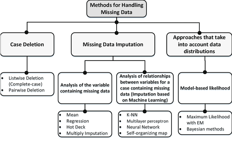
• Handling missing values: Missing values can be handled in several ways, such as mean/mode/median imputation, hot deck imputation, and regression imputation.
• Mean/mode/median imputation involves replacing the missing value with the mean/mode/median of the variable.
• Hot deck imputation involves replacing the missing value with a value from a similar observation.
• Regression imputation involves using a regression model to predict the missing value based on the other variables in the dataset.
• Data Cleaning: Data cleaning involves identifying and removing inaccuracies, inconsistencies, and outliers in the data. This step can improve the quality of the data and increase the accuracy of the analysis.
• Data Transformation: Data transformation involves changing the data in a way that makes it more appropriate for analysis. This can include rescaling data, binarizing data, and feature scaling.
• Rescaling data involves changing the scale of a variable to a standard range, such as 0–1.
• Binarizing data involves converting a variable to a binary format, such as 0 or 1.
• Feature scaling involves changing the scale of a variable so that it has a similar range as the other variables in the dataset.
• Stochastic regression imputation: Stochastic regression imputation is an extension of multiple imputation method, where the imputed values are drawn from the predictive distributions of a regression model. This is done by simulating multiple datasets by drawing imputed values from the posterior predictive distributions of the model.

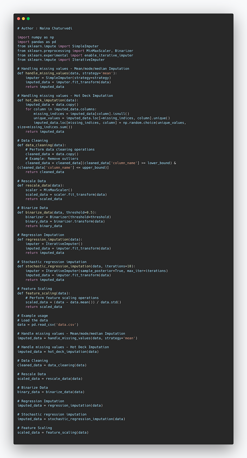
Complete code —

import numpy as np
import pandas as pd
from sklearn.impute import SimpleImputer
from sklearn.preprocessing import MinMaxScaler, Binarizer
from sklearn.experimental import enable_iterative_imputer
from sklearn.impute import IterativeImputer

# Handling missing values - Mean/mode/median Imputation
def handle_missing_values(data, strategy='mean'):
    imputer = SimpleImputer(strategy=strategy)
    imputed_data = imputer.fit_transform(data)
    return imputed_data

# Handling missing values - Hot Deck Imputation
def hot_deck_imputation(data):
    imputed_data = data.copy()
    for column in imputed_data.columns:
        missing_indices = imputed_data[column].isnull()
        unique_values = imputed_data.loc[~missing_indices, column].unique()
        imputed_data.loc[missing_indices, column] = np.random.choice(unique_values, size=missing_indices.sum())
    return imputed_data

# Data Cleaning
def data_cleaning(data):
    # Perform data cleaning operations
    cleaned_data = data.copy()
    # Example: Remove outliers
    cleaned_data = cleaned_data[(cleaned_data['column_name'] >= lower_bound) & (cleaned_data['column_name'] <= upper_bound)]
    return cleaned_data

# Rescale Data
def rescale_data(data):
    scaler = MinMaxScaler()
    scaled_data = scaler.fit_transform(data)
    return scaled_data

# Binarize Data
def binarize_data(data, threshold=0.5):
    binarizer = Binarizer(threshold=threshold)
    binary_data = binarizer.transform(data)
    return binary_data

# Regression Imputation
def regression_imputation(data):
    imputer = IterativeImputer()
    imputed_data = imputer.fit_transform(data)
    return imputed_data

# Stochastic regression imputation
def stochastic_regression_imputation(data, iterations=10):
    imputer = IterativeImputer(sample_posterior=True, max_iter=iterations)
    imputed_data = imputer.fit_transform(data)
    return imputed_data

# Feature Scaling
def feature_scaling(data):
    # Perform feature scaling operations
    scaled_data = (data - data.mean()) / data.std()
    return scaled_data

# Example usage
# Load the data
data = pd.read_csv('data.csv')

# Handle missing values - Mean/mode/median Imputation
imputed_data = handle_missing_values(data, strategy='mean')

# Handle missing values - Hot Deck Imputation
imputed_data = hot_deck_imputation(data)

# Data Cleaning
cleaned_data = data_cleaning(data)

# Rescale Data
scaled_data = rescale_data(data)

# Binarize Data
binary_data = binarize_data(data)

# Regression Imputation
imputed_data = regression_imputation(data)

# Stochastic regression imputation
imputed_data = stochastic_regression_imputation(data)

# Feature Scaling
scaled_data = feature_scaling(data)

Snippet —

Import Libraries

import lib_name as alias_name

Some of the most common libraries we import ( depending on the requirement) —

Numpy : Numpy is a python library for scientific computing — to work with multidimensional array objects and used to handle large amount of data. An array which is a grid of values and is indexed by a tuple of nonnegative integers is main data structure of the Numpy library. ndarray is acronym of N-Dimensional Array.

Pandas : It’s an open source Python package written for the Python programming language for data manipulation, analysis and ML tasks.

Matplotlib : It’s a Python 2D plotting library used to plot any type of charts .

Scikit learn : It’s a library ( largely written in Python, is built upon NumPy, SciPy and Matplotlib) for machine learning which provides efficient tools for ML and statistical modeling including classification, regression, clustering and dimensionality reduction etc.

import numpy as np
import pandas as pd
from matplotlib import pyplot as plt
from sklearn import datasets

Importing Datasets

You can import data as simple as

import pandas as pd
dataset = pd.read_csv('filename.csv')

Or directly load from seaborn or sklearn

sns.load_dataset('iris') #sns is alias for seaborn

For Scikit learn —

from sklearn import datasets
digits = datasets.load_digits()

Handling the missing data values

Missing values, incompleteness, unknown data etc is one of the biggest issues while building machine learning model as it impacts the accuracy.

To handle missing values, we can use Scikit-learn Imputer class of sklearn.preprocessing library.

Implementation —

from sklearn.preprocessing import Imputer
imputer = Imputer(missing_values = 'NaN', strategy = 'mean', axis = 0)
imputer = imputer.fit(X[c:d, a:b])
X[c:d, a:b] = imputer.transform(X[c:d, a:b])

Data cleaning —

Data cleaning is the technique of eliminating garbage, incorrect, duplicate, corrupted, or incomplete data in a dataset as the part of the data preparation process with a motive to build reliable, uniform and standardized data sets. Python pandas is an excellent library for manipulating data and analyzing it.

There are four ways you can perform data cleaning :

1. Drop the missing values
2. Replace the missing values
3. Replace each NaN with a scalar value,
4. Fill the missing values forward or backward.

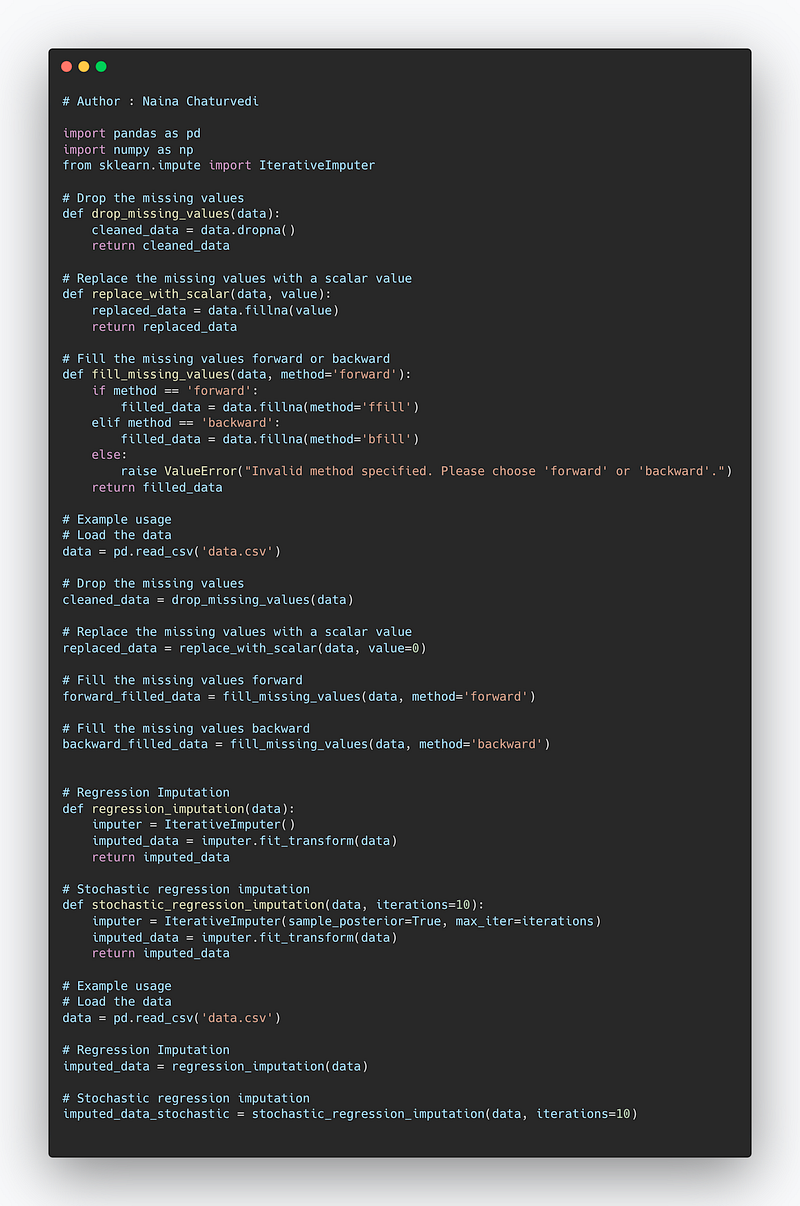
Code Implementation —

import pandas as pd

# Drop the missing values
def drop_missing_values(data):
    cleaned_data = data.dropna()
    return cleaned_data

# Replace the missing values with a scalar value
def replace_with_scalar(data, value):
    replaced_data = data.fillna(value)
    return replaced_data

# Fill the missing values forward or backward
def fill_missing_values(data, method='forward'):
    if method == 'forward':
        filled_data = data.fillna(method='ffill')
    elif method == 'backward':
        filled_data = data.fillna(method='bfill')
    else:
        raise ValueError("Invalid method specified. Please choose 'forward' or 'backward'.")
    return filled_data

# Example usage
# Load the data
data = pd.read_csv('data.csv')

# Drop the missing values
cleaned_data = drop_missing_values(data)

# Replace the missing values with a scalar value
replaced_data = replace_with_scalar(data, value=0)

# Fill the missing values forward
forward_filled_data = fill_missing_values(data, method='forward')

# Fill the missing values backward
backward_filled_data = fill_missing_values(data, method='backward')

Implementation —

Exclude missing values from your dataset using the dropna() method

df.dropna()

Default axis=0 will excludes an entire row for an NaN value.

Replace each NaN we have in the dataset, we can use the replace() method

from numpy import NaN

df.replace({NaN:1.00})

In order to replace with a Scalar Value, use fillna() method

df.fillna(12)

To fill forward or backward, use the methods pad or fill, and to fill backward, use bfill and backfill.

df.fillna(method='backfill')

Mean/mode/median imputation

We can also do mean/median/mode imputation. For numerical data, we can compute it’s mean or median and use the result to replace missing values and for categorical (non-numerical) data, we can compute its mode to replace the missing value.

df.salary.fillna(salary_mean,inplace=True)

Hot Deck Imputation — With this, we can replace the missing value of the observation with a randomly selected value from all the observations in the sample referencing the variables with similar value.

Rescale Data — In order to uniformly scale the attributes with varying scales, rescaling is a useful technique to all have the attributes on the same scale using scikit-learn using the MinMaxScaler class.

# initializing the MinMaxScaler

s_m = MinMaxScaler(feature_range=(0, 2))
rescaledX = s_m.fit_transform(X)

Binarize Data — It’s a very useful process which is generally used during feature engineering to manipulate our data using a binary reference threshold using scikit-learn with the Binarizer class.

b_n = Binarizer(threshold = 1.0).fit(X)
b_X = b_n.transform(X)

Regression Imputation — In order to preserve the relationships between features, we can use regression imputation, basically a technique in which we fit a regression model on a feature with missing data and then using this model predict the values which is used to replace the missing values.

Stochastic regression imputation — In this technique, in order to reproduce the correlation of features and labels, we add a random variation to the predicted value.

Snippet —

Encoding categorical data

Since ML model works on maths and numbers, so it’s necessary we encode these categorical variables into numbers.

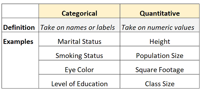
We will use label encoder and One hot encoder ( For Dummy variable Encoding) to accomplish this task.

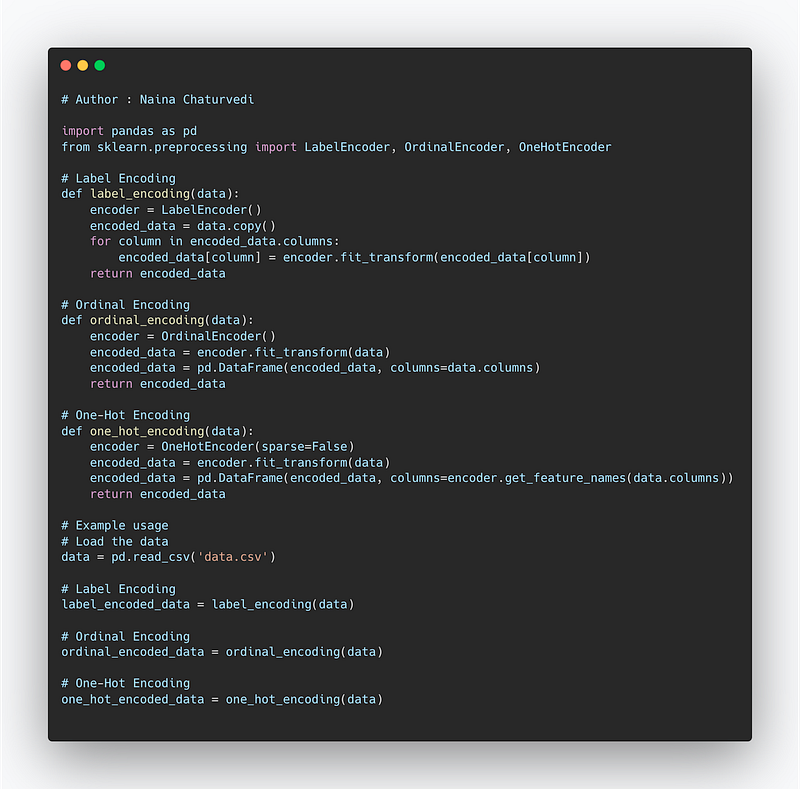
Code Implementation —

# Author : Naina Chaturvedi

import pandas as pd
from sklearn.preprocessing import LabelEncoder, OrdinalEncoder, OneHotEncoder

# Label Encoding
def label_encoding(data):
    encoder = LabelEncoder()
    encoded_data = data.copy()
    for column in encoded_data.columns:
        encoded_data[column] = encoder.fit_transform(encoded_data[column])
    return encoded_data

# Ordinal Encoding
def ordinal_encoding(data):
    encoder = OrdinalEncoder()
    encoded_data = encoder.fit_transform(data)
    encoded_data = pd.DataFrame(encoded_data, columns=data.columns)
    return encoded_data

# One-Hot Encoding
def one_hot_encoding(data):
    encoder = OneHotEncoder(sparse=False)
    encoded_data = encoder.fit_transform(data)
    encoded_data = pd.DataFrame(encoded_data, columns=encoder.get_feature_names(data.columns))
    return encoded_data

# Example usage
# Load the data
data = pd.read_csv('data.csv')

# Label Encoding
label_encoded_data = label_encoding(data)

# Ordinal Encoding
ordinal_encoded_data = ordinal_encoding(data)

# One-Hot Encoding
one_hot_encoded_data = one_hot_encoding(data)

Snippet —

Implementation —

from sklearn.preprocessing import LabelEncoder, OneHotEncoder
labelencoder_X = LabelEncoder()
X[:, 0] = labelencoder_X.fit_transform(X[:, 0]) 
onehotencoder = OneHotEncoder(categorical_features = [0])
X = onehotencoder.fit_transform(X).toarray()
labelencoder_y = LabelEncoder()
y = labelencoder_y.fit_transform(y)

Split Data into Train data and Test data

In order to split arrays/matrices into random train and test subsets, we use train_test_split.

Training data. Used to train the ML model — Feed the algorithm with input data, to give an expected output as the algorithm evaluates the data repeatedly to learn and train with the data and it’s behaviour.

Validation data. Part of training process in which the validation data i.e new data is needed into the model that it hasn’t evaluated before. This data provides the first test against unseen data which helps in evaluating how well the model makes predictions based on the new data and hyperparameter optimization.

Test data. After building the ML model, testing data validates to check if the model makes accurate predictions as well as if it’s trained effectively.

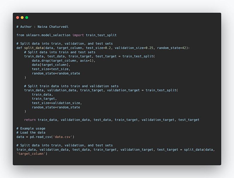
Code Implementation —

from sklearn.model_selection import train_test_split

# Split data into train, validation, and test sets
def split_data(data, target_column, test_size=0.2, validation_size=0.25, random_state=42):
    # Split data into train and test sets
    train_data, test_data, train_target, test_target = train_test_split(
        data.drop(target_column, axis=1),
        data[target_column],
        test_size=test_size,
        random_state=random_state
    )
    
    # Split train data into train and validation sets
    train_data, validation_data, train_target, validation_target = train_test_split(
        train_data,
        train_target,
        test_size=validation_size,
        random_state=random_state
    )
    
    return train_data, validation_data, test_data, train_target, validation_target, test_target

# Example usage
# Load the data
data = pd.read_csv('data.csv')

# Split data into train, validation, and test sets
train_data, validation_data, test_data, train_target, validation_target, test_target = split_data(data, 'target_column')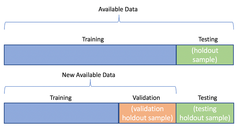

Implementation —

from sklearn.cross_validation import train_test_split
X_train, X_test, y_train, y_test = train_test_split(X, y, test_size = 0.4, random_state = 42)

Where —

x_train: features for the training data

x_test: features for testing data

y_train: Dependent variables for training data

y_test: Independent variable for testing data

random state : to set a seed for a random generator to always get the same result

test_size : to specify the size of the test set

Snippet —

Feature Scaling

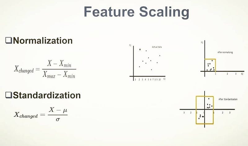
Feature scaling is a technique to standardize the independent variables in the data in a specified range by putting our variables in the same range and scale so that variables don’t dominate each other. It’s important because it always converges and gives results faster.

Normalization also known as Min-Max scaling is a technique in which values in the data are scaled so that they end up ranging between 0 and 1.

Standardization is a technique in which the values are centered around the mean with a unit standard deviation.

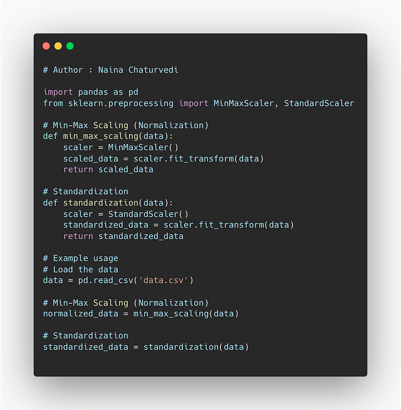
Code Implementation —

import pandas as pd
from sklearn.preprocessing import MinMaxScaler, StandardScaler

# Min-Max Scaling (Normalization)
def min_max_scaling(data):
    scaler = MinMaxScaler()
    scaled_data = scaler.fit_transform(data)
    return scaled_data

# Standardization
def standardization(data):
    scaler = StandardScaler()
    standardized_data = scaler.fit_transform(data)
    return standardized_data

# Example usage
# Load the data
data = pd.read_csv('data.csv')

# Min-Max Scaling (Normalization)
normalized_data = min_max_scaling(data)

# Standardization
standardized_data = standardization(data)

Snippet —

Implementation —

from sklearn.preprocessing import StandardScaler 
ss_X = StandardScaler() 
X_train = ss_X.fit_transform(X_train) 
X_test = ss_X.transform(X_test)

That’s it for now.

Find Day 17 below —

Let me know if you have questions in the comment section below. Subscribe/ Follow, Like/Clap as it would encourage me to write more in my free time

Stay Tuned!!

Read more —

All the Complete System Design Series Parts —

1. System design basics

2. Horizontal and vertical scaling

3. Load balancing and Message queues

4. High level design and low level design, Consistent Hashing, Monolithic and Microservices architecture

5. Caching, Indexing, Proxies

6. Networking, How Browsers work, Content Network Delivery ( CDN)

7. Database Sharding, CAP Theorem, Database schema Design

8. Concurrency, API, Components + OOP + Abstraction

9. Estimation and Planning, Performance

10. Map Reduce, Patterns and Microservices

11. SQL vs NoSQL and Cloud

12. Most Popular System Design Questions

Github —

Keep learning and coding ;)

Day 5 coming soon!

For Python Projects —

For complete 60 days of Data Science and ML : Day 1 — Day 60 : Quick Recap of 60 days of Data Science and ML

Follow for more updates. Stay tuned and keep coding! Disclosure: Some of the links are affiliates.

For other projects, tune to —

Build Machine Learning Pipelines( With Code)

Recurrent Neural Network with Keras

Clustering Geolocation Data in Python using DBSCAN and K-Means

Facial Expression Recognition using Keras

Hyperparameter Tuning with Keras Tuner

Custom Layers in Keras