
Day 8 of 30 days of Data Analytics with Projects Series
Welcome back peeps. Happy to share that we have finished —
Finished Series —
60 Days of Data Science and Machine Learning with projects Series
What’s covered in the Data Analytics Series till now —
Day 1 : Data Analytics basics and kickstart of Data analytics with projects series
Day 3 : Data Analytics Ecosystem — Data Life Cycle, Data Analysis complete process ( most important things)
Day 5 : Statistics
Day 6 : Basic and Advanced SQL
Day 8 : Pandas and Numpy
In the last post we covered part 1 of Data Collection, Data Cleaning and Python. This is part 2 of Data cleaning post as day 8 of Data Analytics Series. In this we will cover —
Pandas
Numpy
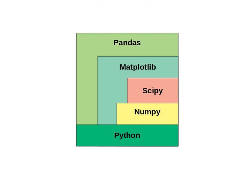
Pandas and NumPy are two popular Python libraries used for data manipulation and analysis.
Projects Videos —
All the projects, data structures, SQL, algorithms, system design, Data Science and ML , Data Analytics, Data Engineering, , Implemented Data Science and ML projects, Implemented Data Engineering Projects, Implemented Deep Learning Projects, Implemented Machine Learning Ops Projects, Implemented Time Series Analysis and Forecasting Projects, Implemented Applied Machine Learning Projects, Implemented Tensorflow and Keras Projects, Implemented PyTorch Projects, Implemented Scikit Learn Projects, Implemented Big Data Projects, Implemented Cloud Machine Learning Projects, Implemented Neural Networks Projects, Implemented OpenCV Projects,Complete ML Research Papers Summarized, Implemented Data Analytics projects, Implemented Data Visualization Projects, Implemented Data Mining Projects, Implemented Natural Leaning Processing Projects, MLOps and Deep Learning, Applied Machine Learning with Projects Series, PyTorch with Projects Series, Tensorflow and Keras with Projects Series, Scikit Learn Series with Projects, Time Series Analysis and Forecasting with Projects Series, ML System Design Case Studies Series videos will be published on our youtube channel ( just launched).
Subscribe today!
Pandas:
- Data structures: Pandas provides two main data structures, the Series (1-dimensional) and DataFrame (2-dimensional), for storing and manipulating data.
- Data cleaning and preprocessing: Pandas has many built-in functions for handling missing values, filtering, and transforming data.
- Data manipulation: Pandas provides powerful methods for merging, grouping, and reshaping data.
- Data visualization: Pandas has built-in support for creating various types of plots and visualizations using the matplotlib library.
Code Implementation —
import pandas as pd
import matplotlib.pyplot as plt

# Data Structures: Series and DataFrame
# Create a Series
series_data = pd.Series([10, 20, 30, 40, 50])
print("Series:")
print(series_data)

# Create a DataFrame
data = {'Name': ['John', 'Alice', 'Bob'],
        'Age': [25, 30, 35],
        'City': ['New York', 'London', 'Paris']}
df = pd.DataFrame(data)
print("\nDataFrame:")
print(df)

# Data Cleaning and Preprocessing
# Handling Missing Values
df['Age'].fillna(df['Age'].mean(), inplace=True)

# Filtering Data
filtered_df = df[df['Age'] > 30]

# Data Manipulation
# Merging DataFrames
data1 = {'Name': ['John', 'Alice'],
         'Salary': [5000, 6000]}
data2 = {'Name': ['Bob', 'Alice'],
         'Department': ['IT', 'Sales']}
df1 = pd.DataFrame(data1)
df2 = pd.DataFrame(data2)
merged_df = pd.merge(df1, df2, on='Name')

# Grouping Data
grouped_df = df.groupby('City')['Age'].mean()

# Data Visualization
df.plot(kind='bar', x='Name', y='Age', legend=False)
plt.xlabel('Name')
plt.ylabel('Age')
plt.title('Age Distribution')
plt.show()
NumPy:
- N-dimensional arrays: NumPy provides the ndarray (n-dimensional array) object for efficient storage and manipulation of large arrays of homogeneous data (e.g., numbers).
- Mathematical operations: NumPy provides many mathematical functions such as trigonometric, logarithmic, and linear algebra functions that can operate on entire arrays.
- Broadcasting: NumPy allows you to perform operations on arrays of different shapes by automatically broadcasting smaller arrays to match the shape of larger arrays.
- Interoperability: NumPy is designed to work seamlessly with other libraries, such as Pandas, and is often used as the underlying data structure for other scientific libraries.
Code Implementation —
import numpy as np

# N-dimensional arrays
# Create a 1-dimensional array
array1d = np.array([1, 2, 3, 4, 5])
print("1-dimensional array:")
print(array1d)

# Create a 2-dimensional array
array2d = np.array([[1, 2, 3], [4, 5, 6]])
print("\n2-dimensional array:")
print(array2d)

# Mathematical operations
# Trigonometric functions
sin_values = np.sin(array1d)
print("\nSin values:")
print(sin_values)

# Logarithmic functions
log_values = np.log(array1d)
print("\nLog values:")
print(log_values)

# Linear algebra functions
matrix1 = np.array([[1, 2], [3, 4]])
matrix2 = np.array([[5, 6], [7, 8]])
matrix_product = np.dot(matrix1, matrix2)
print("\nMatrix product:")
print(matrix_product)

# Broadcasting
array3 = np.array([10, 20, 30])
array_broadcasted = array1d + array3
print("\nBroadcasted array:")
print(array_broadcasted)

# Interoperability
import pandas as pd

data = {'col1': [1, 2, 3, 4, 5],
        'col2': ['A', 'B', 'C', 'D', 'E']}
df = pd.DataFrame(data)

numpy_array = df['col1'].to_numpy()
print("\nNumPy array from DataFrame:")
print(numpy_array)
Output —
1-dimensional array:
[1 2 3 4 5]

2-dimensional array:
[[1 2 3]
 [4 5 6]]

Sin values:
[ 0.84147098  0.90929743  0.14112001 -0.7568025  -0.95892427]

Log values:
[0.         0.69314718 1.09861229 1.38629436 1.60943791]

Matrix product:
[[19 22]
 [43 50]]

Broadcasted array:
[11 22 33 14 25]

NumPy array from DataFrame:
[1 2 3 4 5]
Pandas and NumPy are often used together in data analysis tasks, where Pandas provides the high-level data manipulation functions and NumPy provides the low-level array operations.
Let’s get started.
Pandas
Pandas is a a fast, powerful, flexible and easy to use open source data analysis and manipulation tool. It’s a newer package built on top of NumPy, and provides an efficient implementation of a DataFrame.
Pandas is an open source Python package written for the Python programming language for data manipulation, analysis and ML tasks
It is built on top of another package named Numpy, which provides support for mathematical computations and multi-dimensional arrays.
Here are some of the most important functions in Pandas:
- read_csv() and read_excel(): These functions are used to read in data from a CSV file or Excel file, respectively.
- head() and tail(): These functions are used to return the first or last n rows of a DataFrame, respectively.
- info() and describe(): These functions are used to get information about the DataFrame, such as the number of rows and columns, the data types of each column, and summary statistics.
- drop() and dropna(): These functions are used to remove rows or columns from a DataFrame or to remove rows or columns with missing values, respectively.
- sort_values() and sort_index(): These functions are used to sort the DataFrame by one or more columns or by the index, respectively.
- groupby(): This function is used to group the DataFrame by one or more columns, and then apply a function to each group.
- merge() and join(): These functions are used to combine two DataFrames based on one or more columns, similar to a SQL JOIN operation.
- apply(): This function is used to apply a function to each element of a DataFrame or a Series.
- pivot_table() and crosstab(): These functions are used to create pivot tables, which are a way to summarize and aggregate data in a DataFrame.
- to_csv() and to_excel(): These functions are used to save a DataFrame to a CSV file or Excel file, respectively.
Code Implementation —
import pandas as pd

# Read data from CSV file
df_csv = pd.read_csv('data.csv')

# Read data from Excel file
df_excel = pd.read_excel('data.xlsx')

# Return the first n rows of a DataFrame
first_rows = df_csv.head(5)
print("First 5 rows:")
print(first_rows)

# Return the last n rows of a DataFrame
last_rows = df_excel.tail(3)
print("\nLast 3 rows:")
print(last_rows)

# Get information about the DataFrame
df_info = df_csv.info()
print("\nDataFrame information:")
print(df_info)

# Get summary statistics of the DataFrame
df_desc = df_excel.describe()
print("\nSummary statistics:")
print(df_desc)

# Remove rows or columns from a DataFrame
df_dropped = df_csv.drop(columns=['column1', 'column2'])
print("\nDataFrame with columns dropped:")
print(df_dropped)

# Remove rows with missing values
df_droppedna = df_excel.dropna()
print("\nDataFrame with missing values dropped:")
print(df_droppedna)

# Sort the DataFrame by one or more columns
df_sorted = df_csv.sort_values(by='column1')
print("\nDataFrame sorted by column1:")
print(df_sorted)

# Sort the DataFrame by index
df_sorted_index = df_excel.sort_index()
print("\nDataFrame sorted by index:")
print(df_sorted_index)

# Group the DataFrame by one or more columns and apply a function
df_grouped = df_csv.groupby('column1').sum()
print("\nDataFrame grouped by column1:")
print(df_grouped)

# Merge two DataFrames based on one or more columns
merged_df = pd.merge(df_csv, df_excel, on='common_column')
print("\nMerged DataFrame:")
print(merged_df)

# Apply a function to each element of a DataFrame or a Series
df_applied = df_excel['column1'].apply(lambda x: x * 2)
print("\nApplied function to column1:")
print(df_applied)

# Create a pivot table
pivot_table = pd.pivot_table(df_csv, values='column1', index='column2', columns='column3', aggfunc='sum')
print("\nPivot table:")
print(pivot_table)

# Save DataFrame to a CSV file
df_csv.to_csv('output.csv', index=False)

# Save DataFrame to an Excel file
df_excel.to_excel('output.xlsx', index=False)
Numpy
Numpy is a python library for scientific computing — to work with multidimensional array objects and used to handle large amount of data. An array which is a grid of values and is indexed by a tuple of nonnegative integers is main data structure of the Numpy library.
ndarray is acronym of N-Dimensional Array. We have covered Flattening the arrays, Concatenation and Broadcasting etc in detail in the posts below.
We have covered Pandas and Numpy as the part of MLOps series. In Numpy, you must know —
Code Implementation —
import numpy as np

# Create NumPy arrays
array1 = np.array([1, 2, 3, 4, 5])
array2 = np.array([[1, 2, 3], [4, 5, 6]])
array3 = np.array([1.1, 2.2, 3.3, 4.4, 5.5])

print("NumPy arrays:")
print("Array 1:", array1)
print("Array 2:")
print(array2)
print("Array 3:", array3)

# Zeros arrays
zeros_array = np.zeros((2, 3))
print("\nZeros array:")
print(zeros_array)

# Ones arrays
ones_array = np.ones((3, 2))
print("\nOnes array:")
print(ones_array)

# Full arrays
full_array = np.full((2, 2), 5)
print("\nFull array:")
print(full_array)

# Identity Matrix
identity_matrix = np.eye(3)
print("\nIdentity matrix:")
print(identity_matrix)

# Reshape array
reshaped_array = np.reshape(array1, (5, 1))
print("\nReshaped array:")
print(reshaped_array)

# Flatten array
flattened_array = array2.flatten()
print("\nFlattened array:")
print(flattened_array)

# Concatenation
concatenated_array = np.concatenate((array1, array3))
print("\nConcatenated array:")
print(concatenated_array)

# Broadcasting
broadcasted_array = array1 + 10
print("\nBroadcasted array:")
print(broadcasted_array)

# Scalar product
scalar_product = np.dot(array1, array3)
print("\nScalar product:")
print(scalar_product)
Output —
NumPy arrays:
Array 1: [1 2 3 4 5]
Array 2:
[[1 2 3]
 [4 5 6]]
Array 3: [1.1 2.2 3.3 4.4 5.5]

Zeros array:
[[0. 0. 0.]
 [0. 0. 0.]]

Ones array:
[[1. 1.]
 [1. 1.]
 [1. 1.]]

Full array:
[[5 5]
 [5 5]]

Identity matrix:
[[1. 0. 0.]
 [0. 1. 0.]
 [0. 0. 1.]]

Reshaped array:
[[1]
 [2]
 [3]
 [4]
 [5]]

Flattened array:
[1 2 3 4 5 6]

Concatenated array:
[1. 2. 3. 4. 5. 1.1 2.2 3.3 4.4 5.5]

Broadcasted array:
[11 12 13 14 15]

Scalar product:
66.0
Here are some of the most important functions in NumPy:
- np.array(): This function is used to create a new NumPy array from a Python list or another array-like object.
- np.zeros() and np.ones(): These functions are used to create new arrays filled with zeros or ones, respectively.
- np.shape and np.ndim: These functions are used to get the shape (number of rows and columns) and dimension (number of axes) of an array, respectively.
- np.arange(): This function is used to create a new array with a range of evenly spaced values.
- np.linspace(): This function is used to create a new array with a specified number of evenly spaced values between two endpoints.
- np.random.rand() and np.random.randn(): These functions are used to create new arrays with random values sampled from a uniform or normal distribution, respectively.
- np.min() , np.max(), np.mean(), np.sum(): These functions are used to find the minimum, maximum, mean and sum of array elements
- np.dot() and np.matmul(): These functions are used to perform matrix multiplication on two arrays.
- np.transpose() and np.reshape(): These functions are used to change the shape of an array, transpose flips the array along its diagonal and reshape changes the shape of an array without changing its data
- np.save() and np.load(): These functions are used to save an array to a binary file and load it again later.
Code Implementation —
import numpy as np

# np.array()
arr1 = np.array([1, 2, 3, 4, 5])
print("Array 1:", arr1)

arr2 = np.array([[1, 2, 3], [4, 5, 6]])
print("Array 2:")
print(arr2)

# np.zeros() and np.ones()
zeros_arr = np.zeros((3, 4))
print("Zeros array:")
print(zeros_arr)

ones_arr = np.ones((2, 2))
print("Ones array:")
print(ones_arr)

# np.shape and np.ndim
print("Shape of arr2:", np.shape(arr2))
print("Dimension of arr2:", np.ndim(arr2))

# np.arange()
arr3 = np.arange(1, 10, 2)
print("Array 3 (arange):")
print(arr3)

# np.linspace()
arr4 = np.linspace(0, 1, 5)
print("Array 4 (linspace):")
print(arr4)

# np.random.rand() and np.random.randn()
rand_arr = np.random.rand(2, 3)
print("Random array:")
print(rand_arr)

randn_arr = np.random.randn(2, 3)
print("Random normal array:")
print(randn_arr)

# np.min(), np.max(), np.mean(), np.sum()
print("Minimum value in arr1:", np.min(arr1))
print("Maximum value in arr1:", np.max(arr1))
print("Mean of arr1:", np.mean(arr1))
print("Sum of arr1:", np.sum(arr1))

# np.dot() and np.matmul()
arr5 = np.array([[1, 2], [3, 4]])
arr6 = np.array([[5, 6], [7, 8]])
dot_product = np.dot(arr5, arr6)
matmul_product = np.matmul(arr5, arr6)
print("Dot product:")
print(dot_product)
print("Matrix multiplication:")
print(matmul_product)

# np.transpose() and np.reshape()
transposed_arr2 = np.transpose(arr2)
reshaped_arr1 = np.reshape(arr1, (5, 1))
print("Transposed arr2:")
print(transposed_arr2)
print("Reshaped arr1:")
print(reshaped_arr1)

# np.save() and np.load()
np.save("saved_array", arr1)
loaded_arr = np.load("saved_array.npy")
print("Loaded array:")
print(loaded_arr)
Output —
Array 1: [1 2 3 4 5]
Array 2:
[[1 2 3]
 [4 5 6]]
Zeros array:
[[0. 0. 0. 0.]
 [0. 0. 0. 0.]
 [0. 0. 0. 0.]]
Ones array:
[[1. 1.]
 [1. 1.]]
Shape of arr2: (2, 3)
Dimension of arr2: 2
Array 3 (arange):
[1 3 5 7 9]
Array 4 (linspace):
[0.   0.25 0.5  0.75 1.  ]
Random array:
[[0.53803657 0.80173244 0.31073361]
 [0.10778522 0.20801113 0.84439972]]
Random normal array:
[[ 1.07312543 -0.66341561  0.63715852]
 [ 0.28833208 -0.31339626  1.31250783]]
Minimum value in arr1: 1
Maximum value in arr1: 5
Mean of arr1: 3.0
Sum of arr1: 15
Dot product:
[[19 22]
 [43 50]]
Matrix multiplication:
[[19 22]
 [43 50]]
Transposed arr2:
[[1 4]
 [2 5]
 [3 6]]
Reshaped arr1:
[[1]
 [2]
 [3]
 [4]
 [5]]
Loaded array:
[1 2 3 4 5]
That’s it for now. Day 9 :
Let me know if you have questions in the comment section below. Subscribe/ Follow, Like/Clap as it would encourage me to write more in my free time
Stay Tuned!!
Read More —
11 most important System Design Base Concepts
6. Networking, How Browsers work, Content Network Delivery ( CDN)
13. System Design Template — How to solve any System Design Question
System Design Case Studies — In Depth
Complete Data Structures and Algorithm Series
Some of the other best Series —
30 days of Data Structures and Algorithms and System Design Simplified
Data Science and Machine Learning Research ( papers) Simplified **
100 days : Your Data Science and Machine Learning Degree Series with projects
Complete Data Visualization and Pre-processing Series with projects
Exceptional Github Repos — Part 1
Exceptional Github Repos — Part 2
Tech Newsletter —
If you are interested, you can join my newsletter through which I send tech interview tips, techniques, patterns, hacks — Software Development, ML, Data Science, Startups and Technology projects to more than 30K readers. You can subscribe to Tech Brew :
For Python Projects —
For complete 60 days of Data Science and ML : Day 1 — Day 60 : Quick Recap of 60 days of Data Science and ML
Follow for more updates. Stay tuned and keep coding!
For other projects, tune to —
Build Machine Learning Pipelines( With Code)
Recurrent Neural Network with Keras
Clustering Geolocation Data in Python using DBSCAN and K-Means
Facial Expression Recognition using Keras
Hyperparameter Tuning with Keras Tuner
Custom Layers in Keras


