
Day 12 of 30 days of Data Analytics with Projects Series
Welcome back peeps. This is Day 12 of 30 days of data analytics.
What’s covered in the Data Analytics Series till now —
Day 1 : Data Analytics basics and kickstart of Data analytics with projects series
Day 3 : Data Analytics Ecosystem — Data Life Cycle, Data Analysis complete process ( most important things)
Day 5 : Statistics
Day 6 : Basic and Advanced SQL
Day 8 : Pandas and Numpy
Day 9 : Data Manipulation
Day 10 : Data Visualization — Part 1
Day 11 : Data Visualization — Part 2
Day 12 : Data Visualization — Part 3
In the last post we covered —
Data Visualization — Part 1
In this post we will cover data visualization — part 2 as follows —
Data Visualization — Part 2
Data Visualization using Matplotlib and Seaborn with project
Data Visualization — Part 3
Projects Videos —
All the projects, data structures, SQL, algorithms, system design, Data Science and ML , Data Analytics, Data Engineering, , Implemented Data Science and ML projects, Implemented Data Engineering Projects, Implemented Deep Learning Projects, Implemented Machine Learning Ops Projects, Implemented Time Series Analysis and Forecasting Projects, Implemented Applied Machine Learning Projects, Implemented Tensorflow and Keras Projects, Implemented PyTorch Projects, Implemented Scikit Learn Projects, Implemented Big Data Projects, Implemented Cloud Machine Learning Projects, Implemented Neural Networks Projects, Implemented OpenCV Projects,Complete ML Research Papers Summarized, Implemented Data Analytics projects, Implemented Data Visualization Projects, Implemented Data Mining Projects, Implemented Natural Leaning Processing Projects, MLOps and Deep Learning, Applied Machine Learning with Projects Series, PyTorch with Projects Series, Tensorflow and Keras with Projects Series, Scikit Learn Series with Projects, Time Series Analysis and Forecasting with Projects Series, ML System Design Case Studies Series videos will be published on our youtube channel ( just launched).
Subscribe today!
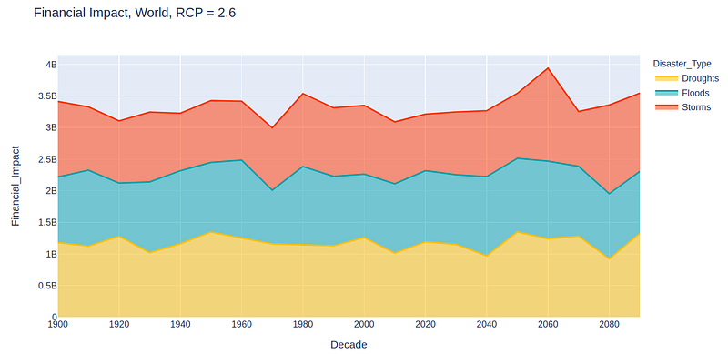
Data Visualization using Plotly
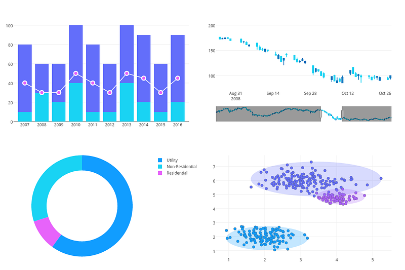
Plotly, built on top of Plotly Graph objects, is a high level data visualization package which allows you to create visualizations that are interactive in nature.
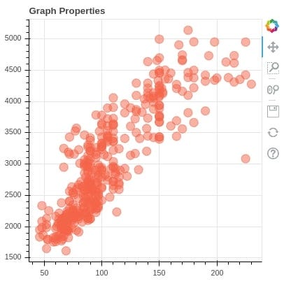
It has interactive controls as shown below —

Using these controls one can —
- Download the chart as png
- Zoom
- Move around the chart
- Select a box region on the chart to be highlighted
- Draw a region of the chart
- Zoom to best scale
- Reset the axes
- Show details on hovering over the chart
To import plotly in your jupyter/colab notebook —
import plotly.express as pxSome of the most important plot types —
- Line plots
px.line(data,x,y)- Scatter plots
px.scatter(data,x,y)- Bar Plots
px.bar(data,x,y,color_map)- Histograms
px.histogram(data,x)- Heatmaps
px.imshow(data.corr(numeric_value),zmin,zmax,color_continuous_scale)One can also customize the lines, markers and bars in Plotly.
To set the lines, you can set the parameters such as—
color
dash
shape
width etc
Example —
line :{"dot",markers = True, "width":8}To set markers, you can set the parameters such as —
size
color
line
symbol etc
markers = {"size" : 12,"color" = "Blue","line" : {"width":1,"color":"black"},
"symbol" = "circle"}
Complete Code —
import plotly.express as px
import plotly.graph_objects as go

# Line Chart
x = [1, 2, 3, 4, 5]
y = [10, 15, 7, 12, 8]
fig = go.Figure(data=go.Scatter(x=x, y=y, mode='lines'))
fig.update_layout(title='Line Chart')
fig.show()

# Column Chart
fig = go.Figure(data=go.Bar(x=x, y=y))
fig.update_layout(title='Column Chart')
fig.show()

# Histogram
data = [1, 1, 2, 2, 2, 3, 3, 4, 5]
fig = px.histogram(data, nbins=5)
fig.update_layout(title='Histogram')
fig.show()

# Bar Chart
fig = go.Figure(data=go.Bar(x=x, y=y, orientation='h'))
fig.update_layout(title='Bar Chart')
fig.show()

# Stacked Column Chart
y2 = [5, 8, 10, 6, 12]
fig = go.Figure()
fig.add_trace(go.Bar(x=x, y=y, name='Value1'))
fig.add_trace(go.Bar(x=x, y=y2, name='Value2'))
fig.update_layout(title='Stacked Column Chart', barmode='stack')
fig.show()

# Pie Chart
labels = ['A', 'B', 'C', 'D', 'E']
values = [10, 15, 7, 12, 8]
fig = px.pie(names=labels, values=values)
fig.update_layout(title='Pie Chart')
fig.show()

# Donut Chart
fig = px.pie(names=labels, values=values, hole=0.4)
fig.update_layout(title='Donut Chart')
fig.show()

# Area Chart
fig = go.Figure(data=go.Scatter(x=x, y=y, mode='lines'))
fig.update_layout(title='Area Chart', yaxis=dict(range=[0, max(y)]))
fig.update_traces(fill='tozeroy')
fig.show()

# Scatter Plot
np.random.seed(0)
x = np.random.randn(100)
y = np.random.randn(100)
fig = go.Figure(data=go.Scatter(x=x, y=y, mode='markers'))
fig.update_layout(title='Scatter Plot')
fig.show()

# Box Plot
data = [np.random.normal(0, std, 100) for std in range(1, 4)]
fig = go.Figure()
for i, d in enumerate(data):
    fig.add_trace(go.Box(y=d, name=f'Data {i+1}'))
fig.update_layout(title='Box Plot')
fig.show()

# KDE Chart
import scipy.stats as stats
data = np.random.randn(1000)
kde = stats.gaussian_kde(data)
x = np.linspace(data.min(), data.max(), 100)
y = kde(x)
fig = go.Figure(data=go.Scatter(x=x, y=y))
fig.update_layout(title='KDE Chart')
fig.show()
Data Visualization using Bokeh
Boken is a interactive visualization library which enables high performance data visualization of large datasets in the browsers.
It’s about two things — data + glyphs which results in a plot.
To get started with bokeh, one needs to —
Load the data
Create the chart
Add renders
Save the results/output the chart file.
Use bokeh.plotting interface as —
from bokeh.plotting import figure
from bokeh.io import output_file,show
For hover glyphs
from bokeh.models import HoverTool
h= HoverTool(tooltips, mode)
Complete Code —
from bokeh.plotting import figure, show
from bokeh.models import ColumnDataSource
from bokeh.palettes import Spectral5
from bokeh.transform import factor_cmap
from bokeh.layouts import gridplot
from bokeh.io import output_notebook
import numpy as np

# Line Chart
output_notebook()
x = np.linspace(0, 2*np.pi, 100)
y = np.sin(x)

p1 = figure(title="Line Chart", width=400, height=300)
p1.line(x, y)
show(p1)

# Column Chart
categories = ['A', 'B', 'C', 'D']
values = [10, 15, 7, 12]

p2 = figure(x_range=categories, title="Column Chart", width=400, height=300)
p2.vbar(categories, top=values, width=0.5)
show(p2)

# Histogram
data = np.random.normal(0, 1, 1000)

p3 = figure(title="Histogram", width=400, height=300)
p3.quad(top=np.histogram(data, bins=30)[0], bottom=0, left=np.histogram(data, bins=30)[1][:-1], right=np.histogram(data, bins=30)[1][1:])
show(p3)

# Bar Chart
p4 = figure(y_range=categories, title="Bar Chart", width=400, height=300)
p4.hbar(y=categories, right=values, height=0.5)
show(p4)

# Stacked Column Chart
data = {'categories': ['A', 'B', 'C', 'D'],
        'value1': [10, 15, 7, 12],
        'value2': [5, 8, 10, 6]}

source = ColumnDataSource(data=data)

p5 = figure(x_range=data['categories'], title="Stacked Column Chart", width=400, height=300)
p5.vbar_stack(stackers=['value1', 'value2'], x='categories', width=0.5, color=['blue', 'red'], source=source)
show(p5)

# Pie Chart
p6 = figure(title="Pie Chart", width=400, height=300)
p6.wedge(x=0, y=0, radius=0.4, start_angle=0, end_angle=np.pi/2, color=["blue", "red", "green", "orange"], legend_label=categories)
show(p6)

# Donut Chart
p7 = figure(title="Donut Chart", width=400, height=300)
p7.wedge(x=0, y=0, radius=0.4, inner_radius=0.2, start_angle=0, end_angle=np.pi/2, color=["blue", "red", "green", "orange"], legend_label=categories)
show(p7)

# Area Chart
p8 = figure(title="Area Chart", width=400, height=300)
p8.patch(x=np.append(x, x[::-1]), y=np.append(y, np.zeros_like(y)), fill_alpha=0.3, line_color="blue")
show(p8)

# Scatter Plot
x = np.random.randn(100)
y = np.random.randn(100)

p9 = figure(title="Scatter Plot", width=400, height=300)
p9.circle(x, y)
show(p9)

# Box Plot
data = [np.random.normal(0, std, 100) for std in range(1, 4)]

p10 = figure(title="Box Plot", width=400, height=300)
p10.boxplot(data, labels=["Data 1", "Data 2", "Data 3"])
show(p10)

# KDE Chart
from scipy.stats import gaussian_kde

data = np.random.randn(1000)
kde = gaussian_kde(data)
x = np.linspace(data.min(), data.max(), 100)
y = kde(x)

p11 = figure(title="KDE Chart", width=400, height=300)
p11.line(x, y)
show(p11)

# Additional Charts
# You can continue to add more charts as needed using the same format

# Gridplot to display all charts together
grid = gridplot([[p1, p2, p3, p4], [p5, p6, p7, p8], [p9, p10, p11]])

show(grid)
In the Day 14 post of 30 days of Data Analytics, we will build a project using Plotly and Bokeh.
That’s it for now. Day 13: Coming Soon!
Let me know if you have questions in the comment section below. Subscribe/ Follow, Like/Clap as it would encourage me to write more in my free time
Stay Tuned!!
Read More —
11 most important System Design Base Concepts
6. Networking, How Browsers work, Content Network Delivery ( CDN)
13. System Design Template — How to solve any System Design Question
System Design Case Studies — In Depth
Complete Data Structures and Algorithm Series
Some of the other best Series —
30 days of Data Structures and Algorithms and System Design Simplified
Data Science and Machine Learning Research ( papers) Simplified **
100 days : Your Data Science and Machine Learning Degree Series with projects
Complete Data Visualization and Pre-processing Series with projects
Exceptional Github Repos — Part 1
Exceptional Github Repos — Part 2
Tech Newsletter —
If you are interested, you can join my newsletter through which I send tech interview tips, techniques, patterns, hacks — Software Development, ML, Data Science, Startups and Technology projects to more than 30K readers. You can subscribe to Tech Brew :
For Python Projects —
For complete 60 days of Data Science and ML : Day 1 — Day 60 : Quick Recap of 60 days of Data Science and ML
Follow for more updates. Stay tuned and keep coding!
For other projects, tune to —
Build Machine Learning Pipelines( With Code)
Recurrent Neural Network with Keras
Clustering Geolocation Data in Python using DBSCAN and K-Means
Facial Expression Recognition using Keras
Hyperparameter Tuning with Keras Tuner
Custom Layers in Keras


