
Project 2— Day 16 of 30 days of Data Analytics with Projects Series
Welcome back peeps. This is Day 16 of 30 days of data analytics where we will be implementing a project.
What’s covered in 30 days of Data Analytics Series till now —
Day 1 : Data Analytics basics and kickstart of Data analytics with projects series
Day 3 : Data Analytics Ecosystem — Data Life Cycle, Data Analysis complete process ( most important things)
Day 5 : Statistics
Day 6 : Basic and Advanced SQL
Day 8 : Pandas and Numpy
Day 9 : Data Manipulation
Day 10 : Data Visualization — Part 1
Day 11 : Project 1 : Data Visualization — Part 2
Day 12 : Data Visualization — Part 3
Day 13: Tableau — Part 1
Day 14: Tableau — Part 2
Day 15: Tableau — Part 3
Day 16 : Data Analysis Project 2
Day 17 : Data Analysis Project 3
Take Complete Hands On Tableau Course : Link
Projects Videos —
All the projects, data structures, SQL, algorithms, system design, Data Science and ML , Data Analytics, Data Engineering, , Implemented Data Science and ML projects, Implemented Data Engineering Projects, Implemented Deep Learning Projects, Implemented Machine Learning Ops Projects, Implemented Time Series Analysis and Forecasting Projects, Implemented Applied Machine Learning Projects, Implemented Tensorflow and Keras Projects, Implemented PyTorch Projects, Implemented Scikit Learn Projects, Implemented Big Data Projects, Implemented Cloud Machine Learning Projects, Implemented Neural Networks Projects, Implemented OpenCV Projects,Complete ML Research Papers Summarized, Implemented Data Analytics projects, Implemented Data Visualization Projects, Implemented Data Mining Projects, Implemented Natural Leaning Processing Projects, MLOps and Deep Learning, Applied Machine Learning with Projects Series, PyTorch with Projects Series, Tensorflow and Keras with Projects Series, Scikit Learn Series with Projects, Time Series Analysis and Forecasting with Projects Series, ML System Design Case Studies Series videos will be published on our youtube channel ( just launched).
Subscribe today!
Tech Newsletter —
If you are interested, you can join my newsletter through which I send tech interview tips, techniques, patterns, hacks — Software Development, ML, Data Science, Startups and Technology projects to more than 30K readers. You can subscribe to Tech Brew :
In the last posts we covered Data Visualization and in this post we will cover data visualization project.
(Note : Zoom all the images)
Import necessary libraries
import numpy as np # linear algebra
import pandas as pd # data processing, CSV file I/O (e.g. pd.read_csv)
import seaborn as sns
from matplotlib import pyplot as plt
from matplotlib.colors import rgb2hex
import matplotlib.cm as cm
import matplotlib.colors
from collections import Counter
cmap2 = cm.get_cmap('twilight',13)
colors1= []
for i in range(cmap2.N):
    rgb= cmap2(i)[:4]
    colors1.append(rgb2hex(rgb))

# Set style
sns.set(style='whitegrid')
Load the data
df = pd.read_csv('/path to file/Data_file.csv',low_memory=False,index_col=0)# Drop duplicates and Null Values
df.drop_duplicates(inplace=True)
df.dropna()Output —
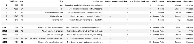
Attribute information —
This dataset includes 23486 rows and 10 feature variables. Each row corresponds to a customer review, and includes the variables:- Clothing ID: Integer Categorical variable that refers to the specific piece being reviewed.
- Age: Positive Integer variable of the reviewers age.
- Title: String variable for the title of the review.
- Review Text: String variable for the review body.
- Rating: Positive Ordinal Integer variable for the product score granted by the customer from 1 Worst, to 5 Best.
- Recommended IND: Binary variable stating where the customer recommends the product where 1 is recommended, 0 is not recommended.
- Positive Feedback Count: Positive Integer documenting the number of other customers who found this review positive.
- Division Name: Categorical name of the product high level division.
- Department Name: Categorical name of the product department name.
- Class Name: Categorical name of the product class name.
# Get to know your datadf.info()Output —
<class 'pandas.core.frame.DataFrame'>
Int64Index: 23486 entries, 0 to 23485
Data columns (total 10 columns):
 #   Column                   Non-Null Count  Dtype
---  ------                   --------------  -----
 0   Clothing ID              23486 non-null  int64
 1   Age                      23486 non-null  int64
 2   Title                    19676 non-null  object
 3   Review Text              22641 non-null  object
 4   Rating                   23486 non-null  int64
 5   Recommended IND          23486 non-null  int64
 6   Positive Feedback Count  23486 non-null  int64
 7   Division Name            23472 non-null  object
 8   Department Name          23472 non-null  object
 9   Class Name               23472 non-null  object
dtypes: int64(5), object(5)
memory usage: 2.0+ MB
# Missing Values
df.isna().sum()Output —
Clothing ID 0
Age 0
Title 3810
Review Text 845
Rating 0
Recommended IND 0
Positive Feedback Count 0
Division Name 14
Department Name 14
Class Name 14
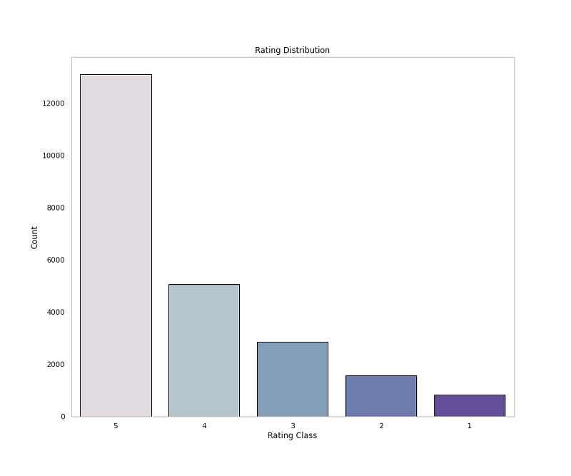
dtype: int64# See the statsdf.describe().T# Get unique Valuesdf.Rating.value_counts()Output —
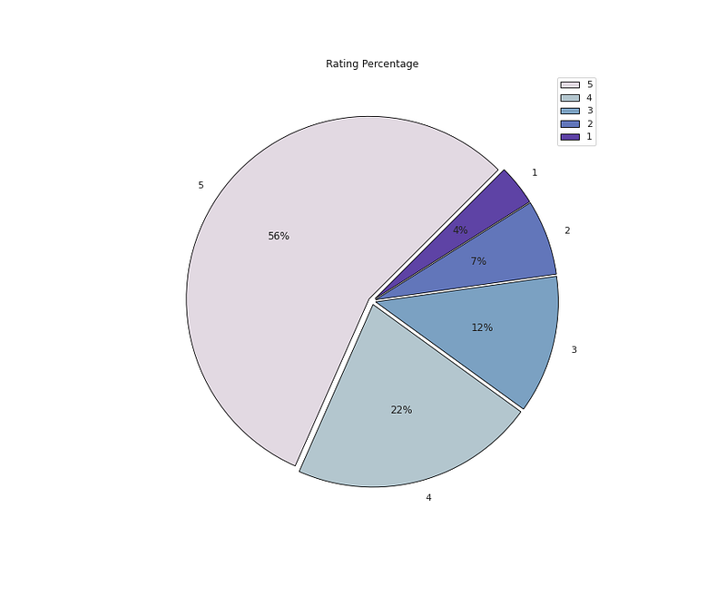
5 13131
4 5077
3 2871
2 1565
1 842
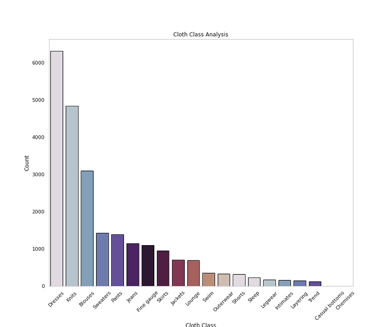
Name: Rating, dtype: int64# Get Class name Countsdf['Class Name'].value_counts()Output —
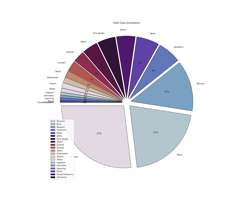
Dresses 6319
Knits 4843
Blouses 3097
Sweaters 1428
Pants 1388
Jeans 1147
Fine gauge 1100
Skirts 945
Jackets 704
Lounge 691
Swim 350
Outerwear 328
Shorts 317
Sleep 228
Legwear 165
Intimates 154
Layering 146
Trend 119
Casual bottoms 2
Chemises 1
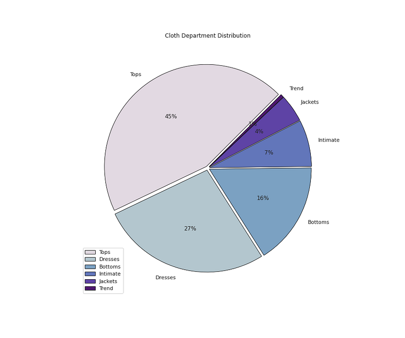
Name: Class Name, dtype: int64# Get Count of Department Namedf['Department Name'].value_counts()Output —
Tops        10468
Dresses      6319
Bottoms      3799
Intimate     1735
Jackets      1032
Trend         119
Name: Department Name, dtype: int64
Data Visualization
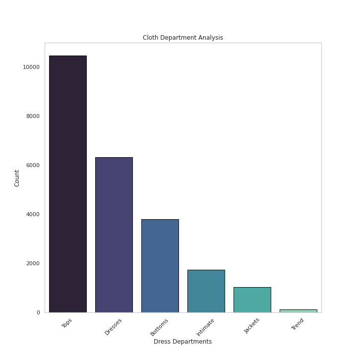
# Cloth Department Analysisplt.figure(figsize=(10,10))
sns.countplot(x='Department Name',data=df,palette='mako',order=df['Department Name'].value_counts().index,edgecolor='black',linewidth=1)
plt.xlabel('Dress Departments')
plt.ylabel('Count')
plt.xticks(rotation=45)
plt.title('Cloth Department Analysis')
plt.grid(False)plt.show()Output —
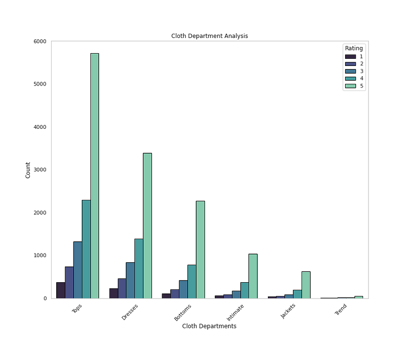
# Cloth Department by Ratingsplt.figure(figsize=(12,10))
sns.countplot(x='Department Name',data=df,palette='mako',order=df['Department Name'].value_counts().index,hue='Rating',edgecolor='black',linewidth=1)
plt.xlabel('Cloth Departments')
plt.ylabel('Count')
plt.xticks(rotation=45)
plt.title('Cloth Department Analysis')
plt.grid(False)plt.show()Output —
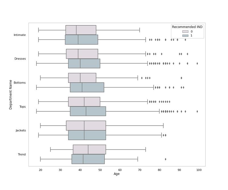
# Cloth Department by Age, Department and Recommendationplt.figure(figsize=(12,10))
sns.boxplot(x = 'Age', y = 'Department Name', data = df,palette=colors1,hue='Recommended IND')
plt.grid(False)plt.title('Cloth Department by Age and Recommendation ')
plt.show()Output —
# Cloth Department Distributionplt.figure(figsize=(12,10))
plt.pie(x=df['Department Name'].value_counts().values,data=df,colors=colors1,labels=df['Department Name'].value_counts().index,autopct='%.0f%%',explode=[0.02 for i in df['Department Name'].value_counts().index],startangle=45,wedgeprops={'linewidth':0.8,'edgecolor':'black'})
plt.title('Cloth Department Distribution')
plt.legend(loc='lower left')plt.show()Output —
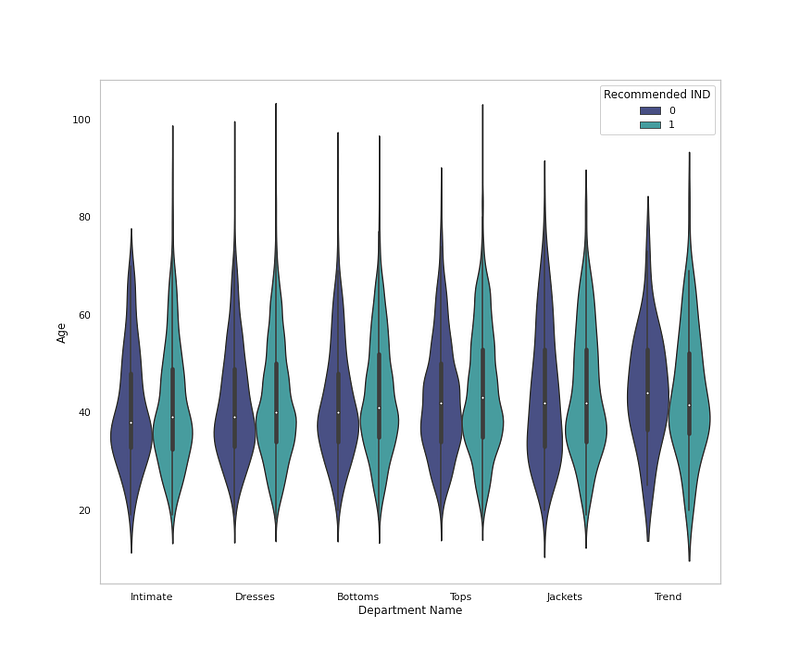
# Cloth Class by Age, Department and Recommendationplt.figure(figsize=(12,10))
sns.violinplot(x = 'Department Name', y = 'Age', data = df,palette='mako',hue='Recommended IND',orient='v')
plt.grid(False)plt.title('Cloth Department by Age and Recommendation ')
plt.show()Output —
# Cloth Class Analysisplt.figure(figsize=(12,10))
sns.countplot(x='Class Name',data=df,palette=colors1,order=df['Class Name'].value_counts().index,edgecolor='black',linewidth=1)
plt.xlabel('Cloth Class')
plt.ylabel('Count')
plt.xticks(rotation=45)
plt.title('Cloth Class Analysis')
plt.grid(False)plt.show()Output —
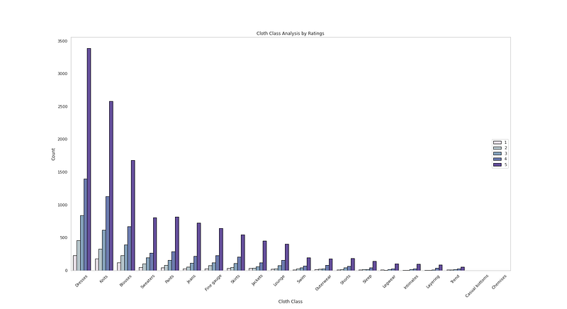
# Cloth Class Analysis by Ratingplt.figure(figsize=(22,12))
sns.countplot(x=df['Class Name'],data=df,palette=colors1,order=df['Class Name'].value_counts().index,edgecolor='black',linewidth=1,hue='Rating')
plt.xlabel('Cloth Class')
plt.ylabel('Count')
plt.xticks(rotation=45)
plt.title('Cloth Class Analysis by Ratings')
plt.grid(False)
plt.legend(loc='right')plt.show()Output —
# Cloth Class Distributionplt.figure(figsize=(18,15))
plt.pie(x=df['Class Name'].value_counts().values,data=df,colors=colors1,labels=df['Class Name'].value_counts().index,autopct='%.0f%%',explode=[0.07 for i in df['Class Name'].value_counts().index],startangle=180,wedgeprops={'linewidth':0.8,'edgecolor':'black'})
plt.title('Cloth Class Distribution')
#plt.grid(False)
plt.legend(loc='lower left')plt.show()Output —
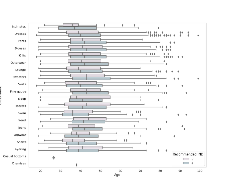
# Cloth Class by Age, Department and Recommendationplt.figure(figsize=(12,10))
sns.boxplot(x = 'Age', y = 'Class Name', data = df,palette=colors1,hue='Recommended IND')
plt.grid(False)plt.title('Cloth Class by Age and Recommendation ')
plt.show()Output —
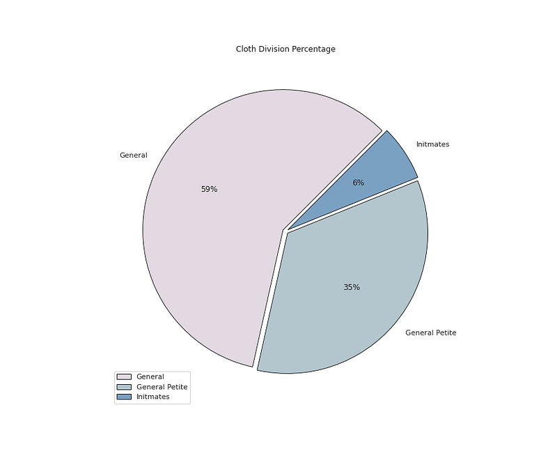
# Division Value Countsdf['Division Name'].value_counts()Output —
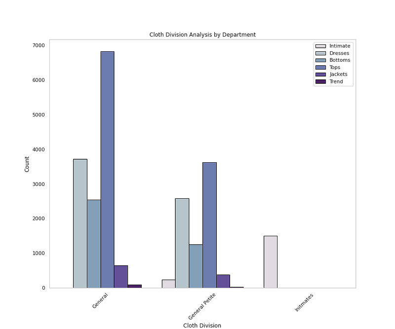
General           13839
General Petite     8110
Initmates          1502
Name: Division Name, dtype: int64
# Cloth Division Analysis by Departmentplt.figure(figsize=(12,10))
sns.countplot(x='Division Name',data=df,palette=colors1,order=df['Division Name'].value_counts().index,edgecolor='black',linewidth=1,hue='Department Name')
plt.xlabel('Cloth Division')
plt.ylabel('Count')
plt.xticks(rotation=45)
plt.title('Cloth Division Analysis by Department')
plt.grid(False)
plt.legend(loc='upper right')plt.show()Output —
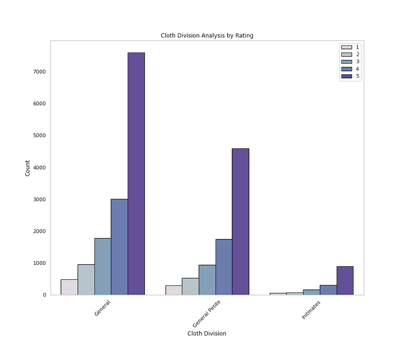
# Cloth Division by Ratingplt.figure(figsize=(12,10))
sns.countplot(x='Division Name',data=df,palette=colors1,order=df['Division Name'].value_counts().index,edgecolor='black',linewidth=1,hue='Rating')
plt.xlabel('Cloth Division')
plt.ylabel('Count')
plt.xticks(rotation=45)
plt.title('Cloth Division Analysis by Rating')
plt.grid(False)
plt.legend(loc='upper right')plt.show()Output —
# Cloth Division Percentageplt.figure(figsize=(12,10))
plt.pie(x=df['Division Name'].value_counts().values,data=df,colors=colors1,labels=df['Division Name'].value_counts().index,autopct='%.0f%%',explode=[0.02 for i in df['Division Name'].value_counts().index],startangle=45,wedgeprops={'linewidth':0.8,'edgecolor':'black'})plt.title('Cloth Division Percentage')plt.legend()
plt.show()Output —
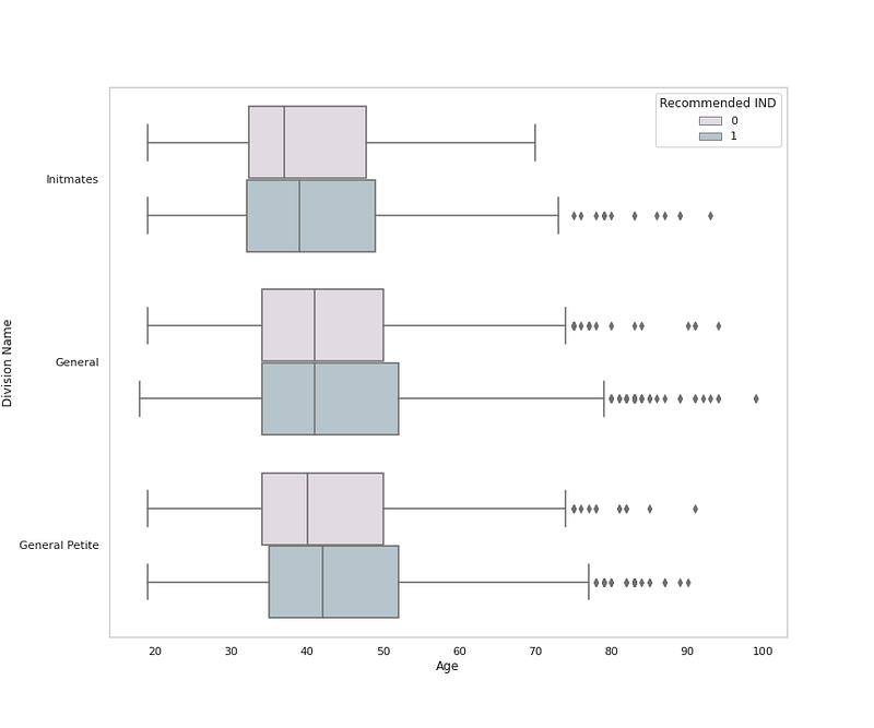
# Cloth Division Name by Ageplt.figure(figsize=(12,10))
sns.boxplot(x = 'Age', y = 'Division Name', data = df,palette=colors1,hue='Recommended IND')
plt.grid(False)plt.title('Cloth Division by Age and Recommendation ')
plt.show()Output —
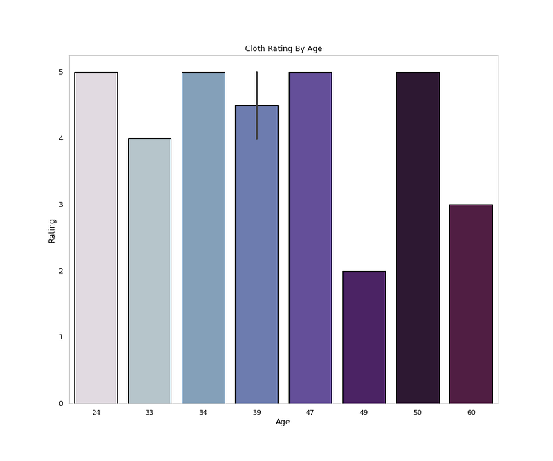
# Rating by Ageplt.figure(figsize=(12,10))
sns.barplot(x=df['Age'].head(10),y='Rating',data=df,palette=colors1,edgecolor='black',linewidth=1)
plt.title('Cloth Rating By Age')
plt.grid(False)plt.show()Output —
# Rating Distributionplt.figure(figsize=(12,10))
sns.countplot(x='Rating',data=df,palette=colors1,order=df['Rating'].value_counts().index,edgecolor='black',linewidth=1)
plt.xlabel('Rating Class')
plt.ylabel('Count')plt.title('Rating Distribution')
plt.grid(False)plt.show()Output —
# Rating Percentageplt.figure(figsize=(12,10))
plt.pie(x=df['Rating'].value_counts().values,data=df,colors=colors1,labels=df['Rating'].value_counts().index,autopct='%.0f%%',explode=[0.02 for i in df['Rating'].value_counts().index],startangle=45,wedgeprops={'linewidth':0.8,'edgecolor':'black'})
plt.title('Rating Percentage')
plt.legend()plt.show()Output —
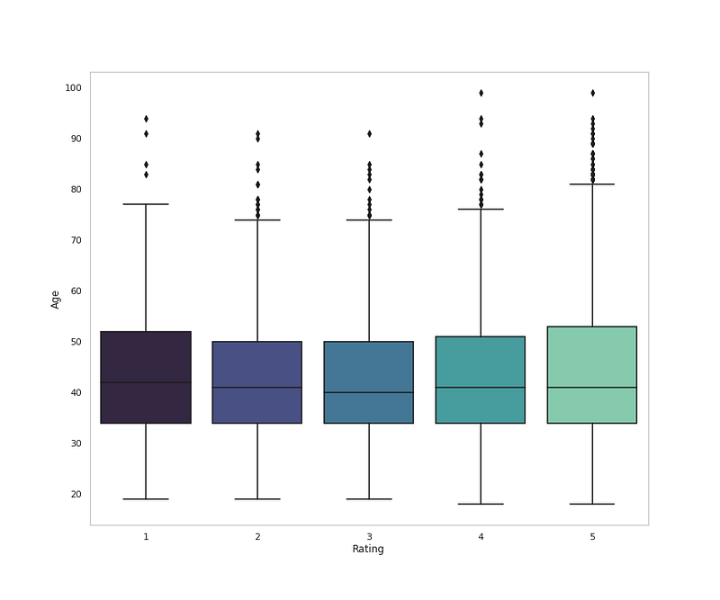
# Rating Distribution by Ageplt.figure(figsize=(12,10))
sns.boxplot(x = 'Rating', y = 'Age', data = df,palette='mako')
plt.grid(False)plt.title('Rating Distribution by Age')
plt.show()Output —
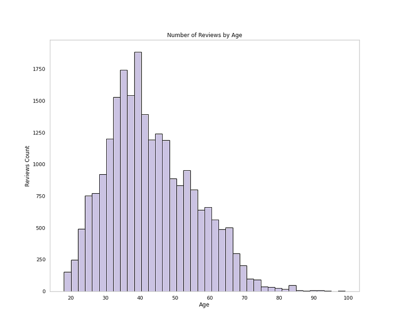
# Age Distributionplt.figure(figsize=(12,10))plt.hist(df['Age'], bins=40,color='#CBC3E3',edgecolor='black')
plt.xlabel('Age')
plt.ylabel('Reviews Count')
plt.grid(False)
plt.title('Number of Reviews by Age')
plt.show()Output —
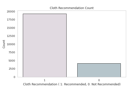
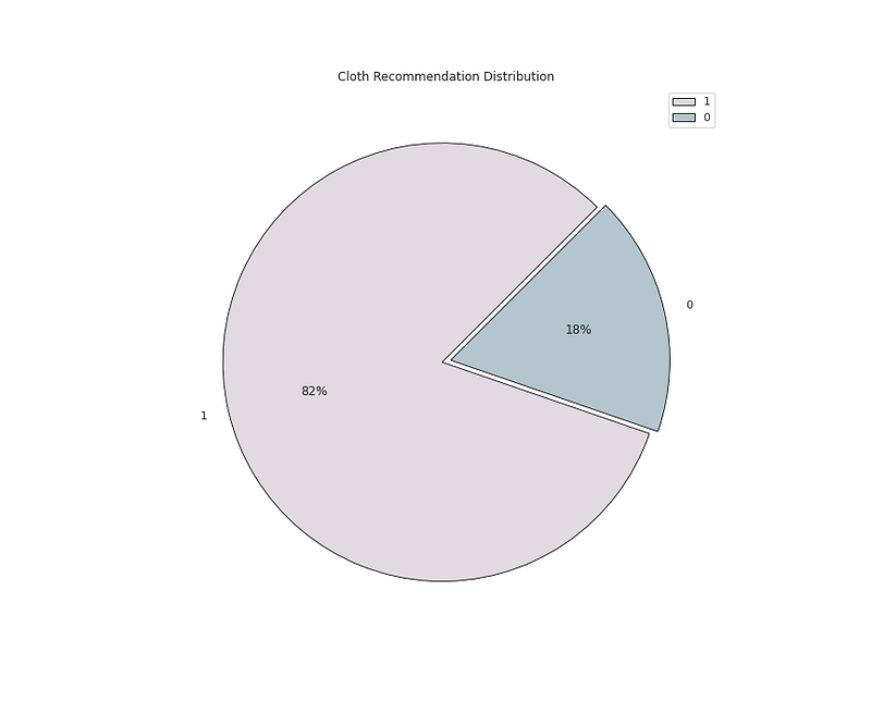
# Cloth Recommendation Analysisdf['Recommended IND'].value_counts()Output —
1 19293
0 4172
Name: Recommended IND, dtype: int64# Cloth Recommendation Countplt.figure(figsize=(8,5))
sns.countplot(x='Recommended IND',data=df,palette=colors1,order=df['Recommended IND'].value_counts().index,edgecolor='black',linewidth=1)
plt.xlabel('Cloth Recommendation ( 1: Recommended, 0: Not Recommended)')
plt.ylabel('Count')plt.title('Cloth Recommendation Count')
plt.grid(False)
plt.show()Output —
# Recommendation Distribution ( 1 means recommended and 0 means not # Recommended by the Customer)plt.figure(figsize=(12,10))
plt.pie(x=df['Recommended IND'].value_counts().values,data=df,colors=colors1,labels=df['Recommended IND'].value_counts().index,autopct='%.0f%%',explode=[0.02 for i in df['Recommended IND'].value_counts().index],startangle=45,wedgeprops={'linewidth':0.8,'edgecolor':'black'})
plt.title('Cloth Recommendation Distribution')
plt.legend()
plt.show()
Output —
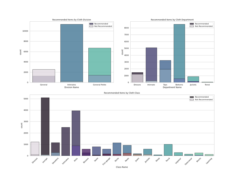
# recommendation Analysis ( 1 means recommended and 0 means not Recommended by the Customer)r = df[df['Recommended IND']==1]
not_r= df[df['Recommended IND']==0]# Plot Cloth Recommendation by Cloth Department, Division, Classfig = plt.figure(figsize=(20, 15))
ax1 = plt.subplot2grid((2, 2), (0, 0))
ax1 = sns.countplot(r['Division Name'], palette ='mako', alpha = 0.8, label = "Recommended",edgecolor='black',linewidth=1)
ax1 = sns.countplot(not_r['Division Name'], palette = colors1, alpha = 0.8, label = "Not Recommended",edgecolor='black',linewidth=1)
ax1 = plt.title("Recommended Items by Cloth Division")
ax1 = plt.legend()ax2 = plt.subplot2grid((2, 2), (0, 1))
ax2 = sns.countplot(r['Department Name'], palette ='mako', alpha = 0.8, label = "Recommended",edgecolor='black',linewidth=1)
ax2 = sns.countplot(not_r['Department Name'], palette =colors1, alpha = 0.8, label = "Not Recommended",edgecolor='black',linewidth=1)
ax2 = plt.title("Recommended Items by Cloth Department")
ax2 = plt.legend()ax3 = plt.subplot2grid((2, 2), (1, 0), colspan=2)
ax3 = plt.xticks(rotation=45)
ax3 = sns.countplot(r['Class Name'], palette ='mako', alpha = 0.8, label = "Recommended",edgecolor='black',linewidth=1)
ax3 = sns.countplot(not_r['Class Name'], palette =colors1, alpha = 0.8, label = "Not Recommended",edgecolor='black',linewidth=1)
ax3 = plt.title("Recommended Items by Cloth Class")
ax3 = plt.legend()plt.show()Output —
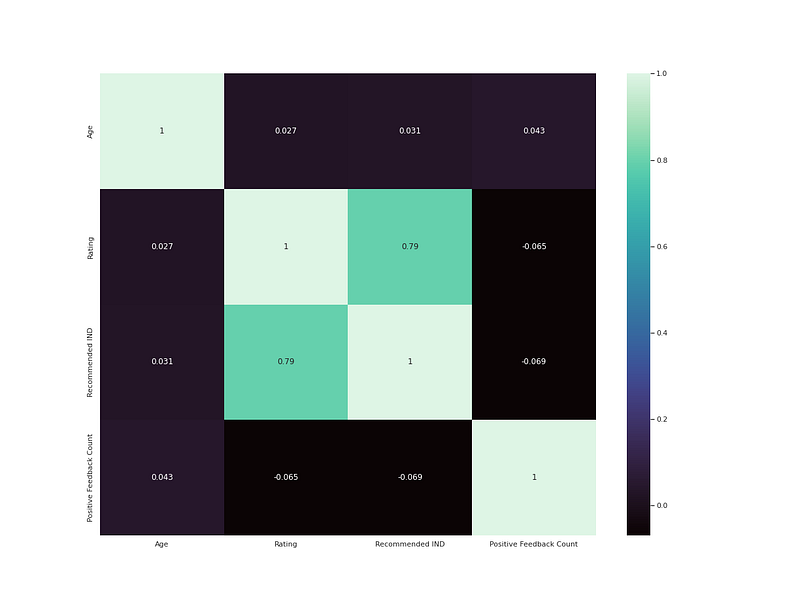
# heatmapplt.figure(figsize=(8,6))
h = df.drop('Clothing ID',axis=1).corr()
sns.heatmap(h,annot=True,cmap='mako')
plt.show()Output —
That’s it for now. Day 17 : Coming Soon!.
Let me know if you have questions in the comment section below. Subscribe/ Follow, Like/Clap as it would encourage me to write more in my free time
Stay Tuned!!
Read More —
11 most important System Design Base Concepts
6. Networking, How Browsers work, Content Network Delivery ( CDN)
13. System Design Template — How to solve any System Design Question
System Design Case Studies — In Depth
Complete Data Structures and Algorithm Series
Some of the other best Series —
30 days of Data Structures and Algorithms and System Design Simplified
Data Science and Machine Learning Research ( papers) Simplified **
100 days : Your Data Science and Machine Learning Degree Series with projects
Complete Data Visualization and Pre-processing Series with projects
Exceptional Github Repos — Part 1
Exceptional Github Repos — Part 2
Tech Newsletter —
If you are interested, you can join my newsletter through which I send tech interview tips, techniques, patterns, hacks — Software Development, ML, Data Science, Startups and Technology projects to more than 30K readers. You can subscribe to Tech Brew :
For Python Projects —
For complete 60 days of Data Science and ML : Day 1 — Day 60 : Quick Recap of 60 days of Data Science and ML
Follow for more updates. Stay tuned and keep coding!
For other projects, tune to —
Build Machine Learning Pipelines( With Code)
Recurrent Neural Network with Keras
Clustering Geolocation Data in Python using DBSCAN and K-Means
Facial Expression Recognition using Keras
Hyperparameter Tuning with Keras Tuner
Custom Layers in Keras


