
Day 5 of 30 days of Data Analytics with Projects Series
Welcome back peeps. Happy to share that we have just finished —
Finished Series —
60 Days of Data Science and Machine Learning with projects Series
Projects Videos —
All the projects, data structures, SQL, algorithms, system design, Data Science and ML , Data Analytics, Data Engineering, , Implemented Data Science and ML projects, Implemented Data Engineering Projects, Implemented Deep Learning Projects, Implemented Machine Learning Ops Projects, Implemented Time Series Analysis and Forecasting Projects, Implemented Applied Machine Learning Projects, Implemented Tensorflow and Keras Projects, Implemented PyTorch Projects, Implemented Scikit Learn Projects, Implemented Big Data Projects, Implemented Cloud Machine Learning Projects, Implemented Neural Networks Projects, Implemented OpenCV Projects,Complete ML Research Papers Summarized, Implemented Data Analytics projects, Implemented Data Visualization Projects, Implemented Data Mining Projects, Implemented Natural Leaning Processing Projects, MLOps and Deep Learning, Applied Machine Learning with Projects Series, PyTorch with Projects Series, Tensorflow and Keras with Projects Series, Scikit Learn Series with Projects, Time Series Analysis and Forecasting with Projects Series, ML System Design Case Studies Series videos will be published on our youtube channel ( just launched).
Subscribe today!
We are now starting a new series — 30 days of Data Analytics with Projects. This series would run in parallel with —
Ongoing Series —
What’s covered till now —
Day 1 : Data Analytics basics and kickstart of Data analytics with projects series
Day 3 : Data Analytics Ecosystem — Data Life Cycle, Data Analysis complete process ( most important things)
Day 5 : Statistics
In the last post we covered Probability and for this post we will cover Statistics.
First understand, Why Statistics?
As we uncover the power of stats, there are numerous questions which stats can help you answer, like ( and the list doesn’t ends here) —
- Ads Targeting and optimization — Which ad is more effective in getting people to purchase a product?
- Optimization — How can you optimize occupancy in a hotel based on the previous occupancy history data?
- Consumer behaviour and insights — How likely is someone to purchase a product? What payment system are they going to use based on their purchasing history data?
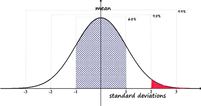
- Patterns — What the most fitting size of t-shirts based on the what 95% of the population is wearing?
Statistics is a field of study that involves the collection, analysis, interpretation, presentation, and organization of data.
To understand statistics, it is important to know the following:
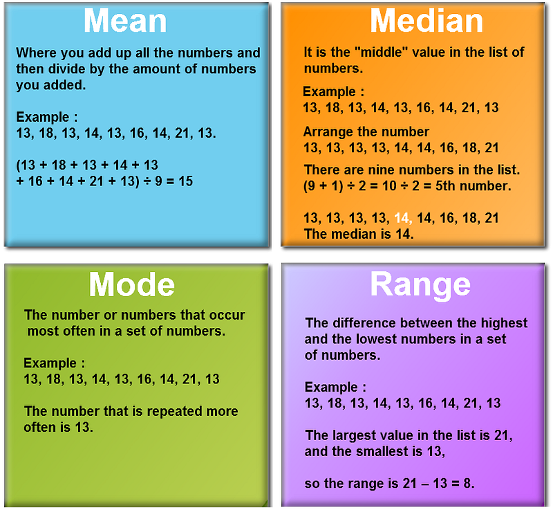
- Descriptive statistics: This involves summarizing and describing the characteristics of a dataset, such as measures of central tendency (mean, median, mode) and measures of dispersion (range, variance, standard deviation).
- Probability: Understanding basic concepts of probability, such as independent and dependent events, conditional probability, and Bayes’ theorem, is essential for statistics.
- Inferential statistics: This involves using a sample of data to make inferences about a population, such as estimation of population parameters and hypothesis testing.
- Data visualization: Visual representation of data using graphs and charts helps to understand and interpret data easily.
- Linear regression and correlation: Linear regression is a statistical method used to study the relationship between two continuous variables. Correlation is used to measure the strength of the relationship between two variables.
- Sampling: Understanding different sampling methods, such as random sampling, stratified sampling, and cluster sampling, is important for collecting data.
- Experimental design: This refers to the planning and execution of experiments, including the control of variables and randomization to minimize bias.
Branches of statistics
Knowing the type of statistics you need to answer your question will help you choose the appropriate methods to get the most accurate answer possible.
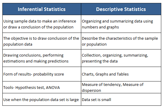
There are two branches of statistics —
Inferential statistics — It takes sample data in order to make inferences with respect to a larger population.
Example —
What % of students drive to college by inferring to the sample data.
import scipy.stats as stats

data = [1, 2, 3, 4, 5]  # Sample data
sample_mean = sum(data) / len(data)  # Sample mean
t_stat, p_value = stats.ttest_1samp(data, population_mean)  # One-sample t-test
confidence_interval = stats.t.interval(0.95, len(data)-1, loc=sample_mean, scale=stats.sem(data))  # Confidence interval
Descriptive statistics — It describes and summarize the data
Example —
How do the students get to their college. Answer can be that 40% of them drive to work, 35% ride the bus, and 25% bike etc.
data = [1, 2, 3, 4, 5]  # Sample data
mean = sum(data) / len(data)  # Mean
median = stats.median(data)  # Median
mode = stats.mode(data)  # Mode
range_val = max(data) - min(data)  # Range
There are two types of data —
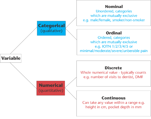
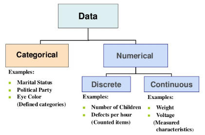
Categorical, or qualitative data: It’s made up of values that belong to distinct groups which is further divided into Nominal and Ordinal. For this type of data we use summary statistics such as counts and plots like barplots etc
Numeric, or quantitative data : It’s made up of numeric values which is further divided into Discrete ( counted items) and Continuous( measured variables). For this type of data we can use summary statistics like mean, and plots like scatter plots etc
Examples of Quantitative Data — Discrete : No of schools, no of children, no of births/hour, Continuous — Weight, Height, Volume etc
Examples of Qualitative data — Marital status, Type of disease, Eye Color etc
Measure of Centre
It’s the value at the center or middle of the data set.
There are four measures of centre —
- Mean- It’s a preferred measure for the interval data
- Median- It’s a preferred measure for the ordinal data
- Mode — It’s a preferred measure for the nominal data
- Range
data = [1, 2, 3, 4, 5]  # Sample data
mean = sum(data) / len(data)  # Mean
median = stats.median(data)  # Median
mode = stats.mode(data)  # Mode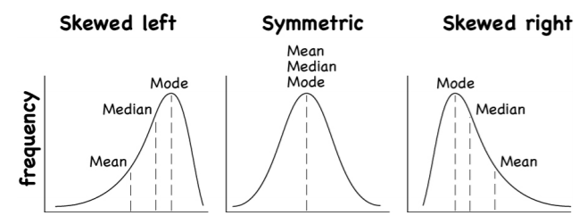
Measure of Spread/ Measure of Variation —
Variability is the key to the statistics. So, when you are describing the data, never rely on the center alone. Measure of spread identified the spread of the values.
There are four measures of spread/variation —
- Standard Deviation
import math

data = [1, 2, 3, 4, 5]  # Sample data
mean = sum(data) / len(data)  # Mean
variance = sum((x - mean) ** 2 for x in data) / len(data)  # Variance
std_dev = math.sqrt(variance)  # Standard deviation
2. Inter-Quartile Range ( IQR)
import numpy as np

data = [1, 2, 3, 4, 5]  # Sample data
q1, q3 = np.percentile(data, [25, 75])  # 1st quartile, 3rd quartile
iqr = q3 - q1  # Inter-quartile range
3. Variance
data = [1, 2, 3, 4, 5]  # Sample data
mean = sum(data) / len(data)  # Mean
variance = sum((x - mean) ** 2 for x in data) / len(data)  # Variance
Measure of frequency : Shows how often a value occurs
Which measure to use?
- If the distribution is normal or symmetrical, use mean and standard deviation. Mean works better for symmetrical data and is more sensitive to extreme values.
- If the distribution is skewed or has large outliers, then use Median, Range or IQR. Median is usually better to use when your data is skewed i.e not symmetrical.
- If the distribution is bimodal, Use mode to figure out if the two modes represent different groups , or range.
Numpy Statistical Functions
Along the specified axis and the given data set , below are the statistical functions that you can use to analyze your data —
np.mean()- To determines the mean value
np.median()- To determines the median value
np.std()- To determines the standard deviation
np.var() — To determines the variance
np.average()- To determines the weighted average
np.percentile()- To determines the nth percentile
np.amin()- To determines the minimum value
np.amax()- To determines the maximum value
Implementation —
import numpy as np
arr1= np.array([[12,43,56],[78,88,95],[79,89,43], [101,34,67]])
arr2 = np.array([5,6,7,12,34,67,89])
#Mean function
print("Mean:", np.mean(arr2))
#Median function
print("Median:",np.median(arr2))
#Standard Deviation Function
print("Standard Deviation:", np.std(arr2))
#Variance Function
print("Variance:",np.var(arr2))
#Average Function
print("Average:",np.average(arr2))
#Percentile Function
print("Percentile:",np.percentile(arr2,5,0))
#Minimum Function
print("Minimum element:",np.amin(arr))
#Maximum Function
print("Maximum element:",np.amax(arr))
Output —
Mean: 31.428571428571427
Median: 12.0
Standard Deviation: 31.409084867994768
Variance: 986.530612244898
Average: 31.428571428571427
Percentile: 5.3
Minimum element: 12
Maximum element: 101
Measure of Spread
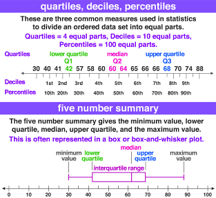
Quantiles are a great way of summarizing numerical data since they can be used to measure center and spread, as well as to get a sense of where a data point stands in relation to the rest of the data set. For example, you might want to give a discount to the 20% most active users on a website.
data = [1, 2, 3, 4, 5]  # Sample data
range_val = max(data) - min(data)  # Range
iqr = stats.iqr(data)  # Inter-quartile range
variance = sum((x - mean) ** 2 for x in data) / len(data)  # Variance
std_dev = math.sqrt(variance)  # Standard deviation
Numpy Quartiles : numpy.quantile(arr, q, axis ) : Compute the qth quantile of the given data
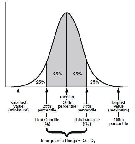
Interquartile range, or IQR, used to measure spread that’s less influenced by outliers and to find the outliers.
If a value is less than Q1−1.5×IQR or greater than Q3+1.5×IQR then it’s considered an outlier.
Calculate the lower and upper cutoffs for outliers
- lower = q1–1.5 * iqr
- upper = q3 + 1.5 * iqr
Implementation —
arr = [31, 35, 45, 49, 59, 69, 74, 79, 80, 81, 89, 94, 96, 99, 101, 104, 112, 117,119,127,134]

# First quartile (Q1)
Q1 = np.median(arr[:12])

# Third quartile (Q3)
Q3 = np.median(arr[12:])

# Interquartile range (IQR)
IQR = Q3 - Q1

print(IQR)
Output —
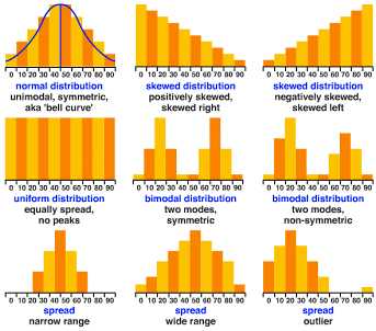
40.5Continuous Probability distribution
Distribution with location (loc) and Scale (scale) parameters.Continuous distributions can be uniform or can take forms where some values have a higher probability than others.
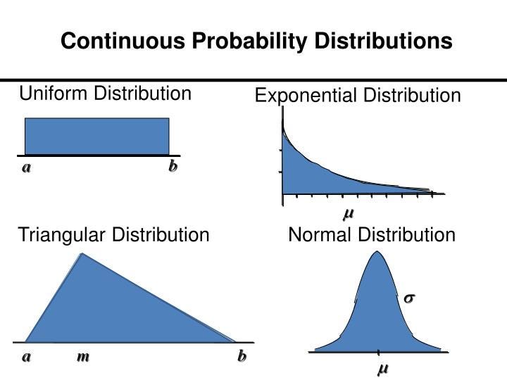
Implementation —
from scipy.stats import uniform
arr2 = np.array([5,6,7,12,34,67,89])
print (uniform.cdf(arr2, loc =4 , scale = 5))
Output —
[0.2 0.4 0.6 1. 1. 1. 1. ]That’s it for now. Day 6:
Let me know if you have questions in the comment section below. Subscribe/ Follow, Like/Clap as it would encourage me to write more in my free time
Stay Tuned!!
Read More —
11 most important System Design Base Concepts
6. Networking, How Browsers work, Content Network Delivery ( CDN)
13. System Design Template — How to solve any System Design Question
System Design Case Studies — In Depth
Complete Data Structures and Algorithm Series
Some of the other best Series —
30 days of Data Structures and Algorithms and System Design Simplified
Data Science and Machine Learning Research ( papers) Simplified **
100 days : Your Data Science and Machine Learning Degree Series with projects
Complete Data Visualization and Pre-processing Series with projects
Exceptional Github Repos — Part 1
Exceptional Github Repos — Part 2
Tech Newsletter —
If you are interested, you can join my newsletter through which I send tech interview tips, techniques, patterns, hacks — Software Development, ML, Data Science, Startups and Technology projects to more than 30K readers. You can subscribe to Tech Brew :
For Python Projects —
For complete 60 days of Data Science and ML : Day 1 — Day 60 : Quick Recap of 60 days of Data Science and ML
Follow for more updates. Stay tuned and keep coding!
For other projects, tune to —
Build Machine Learning Pipelines( With Code)
Recurrent Neural Network with Keras
Clustering Geolocation Data in Python using DBSCAN and K-Means
Facial Expression Recognition using Keras
Hyperparameter Tuning with Keras Tuner
Custom Layers in Keras


