
Stock Time Series Forecasting in a Nutshell: AI/ML Regression/Classification, Statistical Modeling & Cross-Validation QC in Python
Zero to hero use-case examples of learning-based forecasting future stock prices based on historical financial data and various explanatory variables.
“The idea that the future is unpredictable is undermined everyday by the ease with which the past is explained.” — Daniel Kahneman

- In this post, we’ll analyze stock time-series data and build learning-based forecasting models using Python libraries [1–26].
- In the simplest terms, time-series forecasting is a technique that utilizes historical and current data to predict future values over a period of time or a specific point in the future.
- Successful forecast of the future stock price can make considerable profit. According to EMH (efficiency market hypothesis), stock prices reflect all existing information, so any price changes not based on newly released information cannot be forecast.
- The technical goal of this project is to analyze the performance of several widely used forecasting methods in predicting stock market movements: statistical modeling techniques such as Auto-ARIMA [7] and FB Prophet [8–17], supervised Machine Learning (ML) linear/nonlinear regression and binary classification algorithms [1–6, 18] with various explanatory variables or features (time dummy, lags, technical indicators, etc.), and recurrent neural networks with LSTM cells under the umbrella of deep learning as a method in AI [19–24, 26].
- While no forecasting approach can predict stock prices with absolute certainty, these methods can provide useful insights and enable investors to make informed decisions.
- Our business objective is to explore the opportunity of pair trading by predicting high growth US tech stocks (NVDA, TSLA, and AAPL) and the major cryptocurrency such as BTC-USD. Referring to the Macroaxis trading idea, can any of the company-specific risk be diversified away by investing in both tech stocks (e.g. NVDA) and Bitcoin at the same time? Let’s talk about it.
- Key Focus: Trading Strategies Based on Tech Indicators and ML. When ML is being combined with indicators to improve success rates when buying or selling stocks, you can navigate the complexities of the market with efficiency [25].
- Cross-Validation QC Visualization: MAE, MAPE, R2-Score, RMSE, yellowbrick residuals and X-plots (ML Regression); FB Prophet cross-validation metrics; expected returns of ML-based algo-trading strategies (backtesting); ARIMA Validation QC (standardized residuals, histogram plus estimated density, Normal Q-Q plot, and ACF/PACF); feature dominance, correlation matrix, mean accuracy scores, confusion matrix, ROC curve, and full classification reports of supervised ML classification algorithms; ADF/KPSS statistical testing; LSTM MSE Loss vs Epoch curve; Test Time Series Data vs LSTM Predictions.
Contents
- TSLA Linear/Nonlinear Trend Detection with Time Dummy
- TSLA Linear Regression with Lagged Variables
- BTC-USD Price Prediction & Algo-Trading Strategies using FB Prophet
- NVDA Price Prediction using Auto-ARIMA, Supervised ML & Technical Indicators
- BTC-USD Price Prediction using LSTM
- AAPL Price Prediction using LSTM
In the sequel, we’ll delve into the specifics of the aforementioned contents.
TSLA Linear Trend Detection with Time Dummy
- Let’s implement the basic linear regression algorithm using the time dummy as the most basic time-step feature, which counts off time steps in the series from beginning to end [1].
- Reading the input TSLA stock data
import pandas as pd
import yfinance as yf

df_daily =  yf.download('TSLA',
                      start="2024-01-01",
                     progress=False)
df_daily.tail()

           Open       High       Low        Close      Adj Close  Volume
Date
2024-08-28 209.720001 211.839996 202.589996 205.750000 205.750000 64116400
2024-08-29 209.800003 214.889999 205.970001 206.279999 206.279999 62308800
2024-08-30 208.630005 214.570007 207.029999 214.110001 214.110001 63370600
2024-09-03 215.259995 219.899994 209.639999 210.600006 210.600006 76500900
2024-09-04 210.759995 220.399994 210.619995 220.080002 220.080002 29225853 - Preparing the data and training the Linear Regression (LR) model
df1 = df_daily.copy()

df1['Time'] = np.arange(len(df_daily.index))

from sklearn.linear_model import LinearRegression

# Training data
X = df1.loc[:, ['Time']]  # features
y = df1.loc[:, 'Close']  # target

# Train the model
model = LinearRegression()
model.fit(X, y)

# Store the fitted values as a time series with the same time index as
# the training data
y_pred = pd.Series(model.predict(X), index=X.index)

plt.figure(figsize=(10,6))
plt.rcParams.update({'font.size': 12})
ax = y.plot(label='Close Price')
ax = y_pred.plot(ax=ax, linewidth=3,label='Prediction')
ax.set_title('TSLA Linear Regression with Time Dummy');
plt.legend()
plt.ylabel('Price USD')
plt.grid()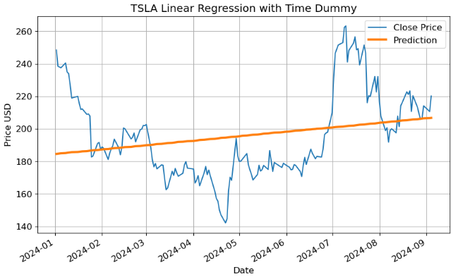
- Calculating the LR performance metrics
from sklearn.metrics import mean_absolute_error, mean_squared_error, r2_score
from sklearn.metrics import mean_absolute_percentage_error
# Calculate MAE, MAPE, R2-Score and RMSE
y_test=y
mae = mean_absolute_error(y_test, y_pred)
rmse = np.sqrt(mean_squared_error(y_test, y_pred))
mape=mean_absolute_percentage_error(y_test, y_pred)
r2score = r2_score(y_test, y_pred)
print(f'Mean Absolute Error: {mae:.2f}')
print(f'MAPE: {mape:.2f}')
print(f'Root Mean Squared Error: {rmse:.2f}')
print(f'R2-Score: {r2score:.2f}')

Mean Absolute Error: 20.58
MAPE: 0.10
Root Mean Squared Error: 25.59
R2-Score: 0.06
Inferences:
- Provided the time series doesn’t have any missing dates, we can create a time dummy by counting out the length of the series.
- The above model assumes a linear relationship [2] between the time variable and Close price. In the current study, this assumption is violated, leading to biased predictions of TSLA stock prices.
TSLA Nonlinear Trend Detection with Time Dummy
- To address the aforementioned drawback of LR, we consider Polynomial Regression (PR) [3, 4] in which the relationship between the time dummy and Close price is modeled as an nth-degree polynomial.
- Running the polynomial regression with n=3
from sklearn.preprocessing import PolynomialFeatures
poly_regressor = PolynomialFeatures(degree=3)

X_columns = poly_regressor.fit_transform(X)

from sklearn.linear_model import LinearRegression
model = LinearRegression()

model.fit(X_columns, y)

pred = model.predict(poly_regressor.fit_transform(X))

plt.figure(figsize=(10,6))
plt.rcParams.update({'font.size': 12})
plt.plot(X, y, color = 'blue',label='Close Price')
plt.plot(X, pred, color = 'red',label='Prediction',lw=3)
plt.ylabel('Price USD')
plt.xlabel('Day Number')
plt.legend(loc='lower right')
plt.title('TSLA Polynomial Regression (degree=3) with Time Dummy')
plt.grid()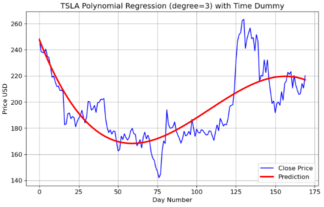
- Calculating the PR performance metrics
# Calculate MAE, MAPE, R2-Score and RMSE
y_test=y
y_pred=pred
mae = mean_absolute_error(y_test, y_pred)
rmse = np.sqrt(mean_squared_error(y_test, y_pred))
mape=mean_absolute_percentage_error(y_test, y_pred)
r2score = r2_score(y_test, y_pred)
print(f'Mean Absolute Error: {mae:.2f}')
print(f'MAPE: {mape:.2f}')
print(f'Root Mean Squared Error: {rmse:.2f}')
print(f'R2-Score: {r2score:.2f}')

Mean Absolute Error: 12.37
MAPE: 0.06
Root Mean Squared Error: 16.52
R2-Score: 0.61
Inferences:
- We can see that PR provides more accurate predictions of TSLA prices than LR.
- The degree of the polynomial equation determines the level of nonlinearity in the price-time relationship.
- However, PR models have poor interpolatory and extrapolatory properties. Even a single outlier in the data can seriously mess up the results. Generally, high degree polynomials (n>>2) are notorious for oscillations between exact-fit values.
TSLA Linear Regression with Lagged Variables
- Our next step is to analyze the impact of lagged features in LR [5–7]. Lagged features will be created by shifting the time series, and a simple LR model will be trained to predict TSLA Close price based on these features, viz.
- Read and explore the TSLA historical data using yfinance
- Transform the dataset to include lagged features (LF) by shifting the time series and examine LF-price correlation coefficients
- Split the input dataset into train/test sets and train a LR model
- Calculate model performance metrics for test data and visualize the regression results using yellowbrick.
- Reading the input TSLA stock data 2022–2024
import pandas as pd
import yfinance as yf


df_daily =  yf.download('TSLA',
                      start="2022-01-01",
                     progress=False)
df_daily.tail()

           Open       High       Low        Close      Adj Close  Volume
Date
2024-08-28 209.720001 211.839996 202.589996 205.750000 205.750000 64116400
2024-08-29 209.800003 214.889999 205.970001 206.279999 206.279999 62308800
2024-08-30 208.630005 214.570007 207.029999 214.110001 214.110001 63370600
2024-09-03 215.259995 219.899994 209.639999 210.600006 210.600006 76500900
2024-09-04 210.759995 222.220001 210.619995 217.639999 217.639999 69155198

data=df_daily.copy()- Plotting PACF of the Close price
from statsmodels.graphics.tsaplots import plot_pacf
series = data['Close']
plot_pacf(series)
plt.show()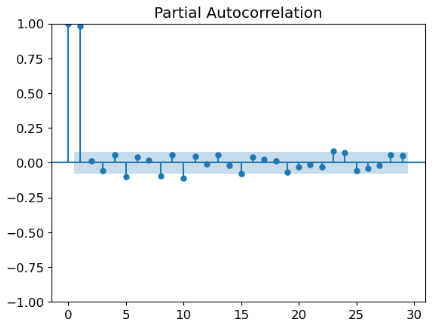
- The above PACF is helpful for identifying lags of the time variable that might be useful predictors of prices.
- Adding LF to the input DataFrame and dropping NaN values [7]
# Adding lag features to the DataFrame
for i in range(1, 6):  # Creating lag features up to 5 days
    data[f'Lag_{i}'] = data['Close'].shift(i)

# Drop rows with NaN values resulting from creating lag features
data.dropna(inplace=True)

data.tail()

           Open       High       Low        Close      Adj Close   Volume   Lag_1      Lag_2      Lag_3      Lag_4      Lag_5
Date
2024-08-28 209.720001 211.839996 202.589996 205.750000 205.750000 64116400 209.210007 213.210007 220.320007 210.660004 223.270004
2024-08-29 209.800003 214.889999 205.970001 206.279999 206.279999 62308800 205.750000 209.210007 213.210007 220.320007 210.660004
2024-08-30 208.630005 214.570007 207.029999 214.110001 214.110001 63370600 206.279999 205.750000 209.210007 213.210007 220.320007
2024-09-03 215.259995 219.899994 209.639999 210.600006 210.600006 76500900 214.110001 206.279999 205.750000 209.210007 213.210007
2024-09-04 210.759995 222.220001 210.619995 218.779999 218.779999 67416126 210.600006 214.110001 206.279999 205.750000 209.210007- Examining the Pearson’s correlation coefficient (CC) between LF (Lag_n, n>0) and Close price (Lag_0)
x=data['Lag_1']
y=data['Close']
r = np.corrcoef(x, y)
print(r[0, 1])
0.9862943483049603

plt.scatter(x,y)
plt.plot(x,x,c='r',lw=3)
plt.xlabel('Lag_1 Close Price')
plt.ylabel('Lag_0 Close Price')
plt.show()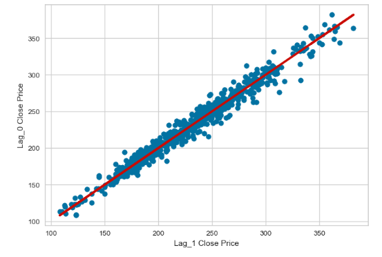
x=data['Lag_2']
y=data['Close']
r = np.corrcoef(x, y)
print(r[0, 1])
0.9738195265814875

plt.scatter(x,y)
plt.plot(x,x,c='r',lw=3)
plt.xlabel('Lag_2 Close Price')
plt.ylabel('Lag_0 Close Price')
plt.show()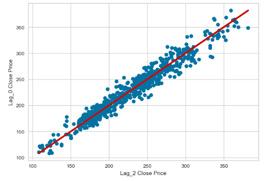
x=data['Lag_3']
y=data['Close']
r = np.corrcoef(x, y)
print(r[0, 1])
0.960646796452951

plt.scatter(x,y)
plt.plot(x,x,c='r',lw=3)
plt.xlabel('Lag_3 Close Price')
plt.ylabel('Lag_0 Close Price')
plt.show()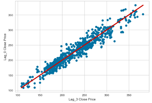
x=data['Lag_4']
y=data['Close']
r = np.corrcoef(x, y)
print(r[0, 1])
0.9486244863366714

plt.scatter(x,y)
plt.plot(x,x,c='r',lw=3)
plt.xlabel('Lag_4 Close Price')
plt.ylabel('Lag_0 Close Price')
plt.show()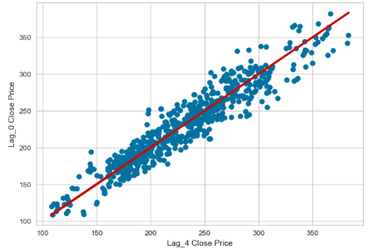
x=data['Lag_5']
y=data['Close']
r = np.corrcoef(x, y)
print(r[0, 1])
0.9335105839215305

plt.scatter(x,y)
plt.plot(x,x,c='r',lw=3)
plt.xlabel('Lag_5 Close Price')
plt.ylabel('Lag_0 Close Price')
plt.show()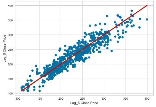
- All five lags are statistically significant with CC>90%.
- Defining the explanatory and dependent variables
X = data[['Lag_1','Lag_2','Lag_3','Lag_4','Lag_5']]  # Features
y = data['Close'] # Target variable - Splitting the dataset into train/test sets with split_ratio = 0.8
split_ratio = 0.8
split_index = int(len(data) * split_ratio)
X_train, X_test = X[:split_index], X[split_index:]
y_train, y_test = y[:split_index], y[split_index:]- Training the LR model and making test predictions
from sklearn.linear_model import LinearRegression
# Train the linear regression model
model = LinearRegression()
model.fit(X_train, y_train)

# Make predictions
predictions = model.predict(X_test)- Calculating the key LR model performance metrics
from sklearn.metrics import mean_absolute_error, mean_squared_error, r2_score
from sklearn.metrics import mean_absolute_percentage_error

mae = mean_absolute_error(y_test, predictions)
mape=mean_absolute_percentage_error(y_test, predictions)
mse = mean_squared_error(y_test, predictions)
r2 = r2_score(y_test, predictions)

MAE: 5.59
MAPE: 0.03
MSE: 56.30
R^2 Score: 0.92- Directly comparing test LR predictions vs Close price
plt.figure(figsize=(10, 6))
plt.plot(y_test,label='Close Price')
plt.plot(y_test.index,predictions,label='Predictions')
plt.xlabel('Date')
plt.ylabel('Price')
plt.title('TSLA Close Price Test Data')
plt.legend()
plt.grid(color='grey')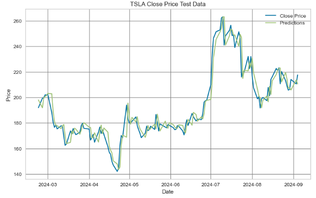
- The above plot shows the actual values of the real time series compared to the predicted values from the LR model. We can see that the predicted values do not deviate significantly from the actual test values.
- Plotting train/test data residuals for the LR model
!pip install yellowbrick

from yellowbrick.regressor import ResidualsPlot

viz = ResidualsPlot(model,
                    train_color="dodgerblue",
                    test_color="tomato",
                    fig=plt.figure(figsize=(9,6))
                    )

viz.fit(X_train, y_train)
viz.score(X_test, y_test)
viz.show();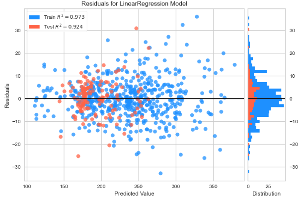
- Plotting test data prediction errors for the LR model
from yellowbrick.regressor import PredictionError


viz = PredictionError(model,
                      fig=plt.figure(figsize=(6,6))
                      )

viz.fit(X_train, y_train)
viz.score(X_test, y_test)
viz.show();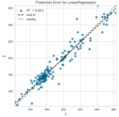
Inferences:
- We have evaluated the LR model that captures the dynamic causal link between an observed stock price and several lagged observations (previous time steps). The core idea is that the current value of a time series can be expressed as a linear combination of its past values, with some random noise [5–7].
- Direct comparisons of the actual time series (i.e. test values against the test predictions), train/test data residuals for the LR model, and X-plots predictions vs test data predicted values do not deviate significantly from the actual test values.
- The following performance metrics give us a quantitative measure of how well the LR model predicts the time series data based on its lagged features
MAE: 5.59
MAPE: 0.03
MSE: 56.30
R^2 Score: 0.92- This result suggests that the LR model fits the Close price quite well and is a good predictor for the TSLA dataset.
BTC-USD Price Prediction & Algo-Trading Strategies using FB Prophet
- In this section, we’ll discuss the BTC-USD price prediction using FB Prophet [8–17], including hyperparameter optimization (HPO), cross-validation QC & modified algo-trading strategies.
- Installation:
!pip install prophet
- Objective: This study focuses on using the FB Prophet framework to forecast BTC-USD prices accurately. By analyzing historical BTC-USD price data, the study aims to capture patterns and dependencies to provide valuable predictive models and profitable algo-trading strategies for investors, traders, and analysts in the volatile cryptocurrency market.
- Challenge: The price of BTC-USD is known for its volatility, which means it can experience significant and rapid fluctuations in a short period. This volatility is characteristic of many cryptocurrencies and is influenced by various factors, such as market friction, regulatory developments, global economic conditions, and investor sentiment.
- Why FB Prophet: A native handling of trend and seasonality features, that makes Prophet a good baseline model if the time series follows business cycles [14]. A great advantage compared to autoregressive models (eg. ARIMA) is that Prophet doesn’t require stationary time series: a trend component is generated natively.
- Let’s delve in further to the matter.
2022–2025 Time Horizon
- Importing the necessary Python libraries
import pandas as pd
import plotly.express as px
import os
os.chdir('YOURPATH')    # Set working directory
os. getcwd()

import requests
import numpy as np
import matplotlib.pyplot as plt
from math import floor
from termcolor import colored as cl


plt.rcParams['figure.figsize'] = (12, 6)
plt.style.use('fivethirtyeight')

import pandas as pd
import yfinance as yf
import datetime
from datetime import date, timedelta
from plotly.subplots import make_subplots
import plotly.graph_objects as go
from datetime import datetime

today = date.today()- Reading and plotting the BTC-USD historical data
d1 = today.strftime("%Y-%m-%d")
end_date = d1
d2 = date.today() - timedelta(days=730)
d2 = d2.strftime("%Y-%m-%d")
start_date = d2

data = yf.download('BTC-USD',
                      start=start_date,
                      end=end_date,
                      progress=False)
data["Date"] = data.index
data = data[["Date", "Open", "High", "Low", "Close", "Adj Close", "Volume"]]
data.reset_index(drop=True, inplace=True)
data.tail()

Date           Open      High      Low       Close     Adj Close Volume
725 2024-08-31 59,117.48 59,432.59 58,768.79 58,969.90 58,969.90 12403470760
726 2024-09-01 58,969.80 59,062.07 57,217.82 57,325.49 57,325.49 24592449997
727 2024-09-02 57,326.97 59,403.07 57,136.03 59,112.48 59,112.48 27036454524
728 2024-09-03 59,106.19 59,815.06 57,425.17 57,431.02 57,431.02 26666961053
729 2024-09-04 57,430.35 58,511.57 55,673.16 57,971.54 57,971.54 35627680312

plt.plot(data['Date'],data['Close'])
plt.xlabel('Date')
plt.ylabel('Close Price USD')
plt.title('BTC-USD Close Price')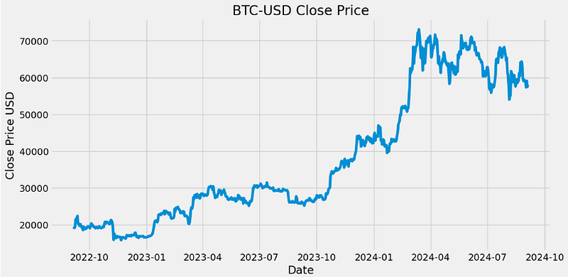
- Plotting the BTC-USD candlesticks with the 20-, 40-day simple moving averages, volume and the volatility histogram in Plotly [15]
class StockAnalysis:
def __init__(self, symbol, source, start, end=datetime.today().strftime('%Y-%m-%d')):
self.symbol = symbol
self.source = source
self.start = start
self.end = end
self.data = None
def fetch_prepare_data(self):
"""
Fetch historical data from the specified source, filter out days without trading activity,
and calculate moving averages. Currently, supports Yahoo Finance via yfinance.
"""
try:
if self.source.lower() == 'yahoo':
data = yf.download(self.symbol, start=self.start, end=self.end)
else:
raise ValueError("Currently, only 'yahoo' source is supported.")
except ValueError as e:
print(f"Error: {e}")
return
except Exception as e:
print(f"An error occurred while fetching data: {e}")
return
self.data = data
return data
def generate_plot(self):
"""
Generate and display a candlestick chart with MA20, MA40, and volume.
"""
self.data['MA20'] = self.data['Close'].rolling(window=20).mean()
self.data['MA40'] = self.data['Close'].rolling(window=40).mean()
try:
# Initialize a figure with subplots
fig = make_subplots(rows=2, cols=1,
shared_xaxes=True,
vertical_spacing=0.15,
subplot_titles=(f'{self.symbol}', ''),
row_width=[0.2, 0.7]
)
# Add Candlestick plot
fig.add_trace(go.Candlestick(x=self.data.index, open=self.data['Open'], high=self.data['High'],
low=self.data['Low'], close=self.data['Close'], name="Candlestick",
increasing_line_color='green', decreasing_line_color='red'), row=1, col=1)
# Add MA20 and MA40
fig.add_trace(go.Scatter(x=self.data.index, y=self.data['MA20'], mode='lines',
line=dict(color='blue', width=1.5), name='MA 20'), row=1, col=1)
fig.add_trace(go.Scatter(x=self.data.index, y=self.data['MA40'], mode='lines',
line=dict(color='orange', width=1.5), name='MA 40'), row=1, col=1)
# Add Volume plot
colors = ['green' if row['Close'] > row['Open'] else 'red' for index, row in self.data.iterrows()]
fig.add_trace(go.Bar(x=self.data.index, y=self.data['Volume'], name='', marker_color=colors), row=2,
col=1)
# Find the first available dates in January and June
tickvals = []
ticktext = []
for year in range(int(self.start[:4]), int(self.end[:4]) + 1):
for month in [1, 6]: # January and June
month_data = self.data[(self.data.index.month == month) & (self.data.index.year == year)]
if not month_data.empty:
first_date = month_data.index[0]
tickvals.append(first_date)
ticktext.append(first_date.strftime('%Y-%m-%d'))
# Set x-axis type to 'category' and specify tickvals and ticktext
fig.update_xaxes(type='category', tickvals=tickvals, ticktext=ticktext)
# Update layout and show the figure as before...
fig.update_layout(title=f'{self.symbol} Candlestick Chart with MA20, MA40, and Volume',
xaxis_title='', yaxis_title='',
template='plotly_white', showlegend=False,
margin=dict(b=80))
return fig
except Exception as e:
print(f"An error occurred during plot generation: {e}")
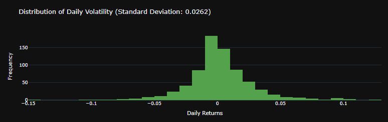
def generate_volatility_histogram(self):
"""
Generate and display a histogram of daily volatility.
"""
try:
# Calculate daily returns
self.data['Daily Return'] = self.data['Close'].pct_change()
# Compute daily volatility (standard deviation of daily returns)
daily_volatility = self.data['Daily Return'].std()
# Plot histogram of daily volatility
fig = go.Figure(data=[go.Histogram(x=self.data['Daily Return'], nbinsx=50, marker_color='#54A24B')])
fig.update_layout(title=f'Distribution of Daily Volatility\n(Standard Deviation: {daily_volatility:.4f})',
xaxis_title='Daily Returns',
yaxis_title='Frequency',
template='plotly_dark')
return fig
except Exception as e:
print(f"An error occurred during plot generation: {e}")
analysis = StockAnalysis(symbol='BTC-USD', source = 'yahoo', start =d2)
data = analysis.fetch_prepare_data()
fig_candelestick = analysis.generate_plot()
fig_candelestick.show()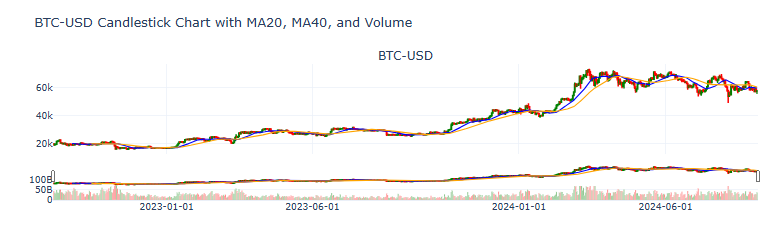
fig_volatility = analysis.generate_volatility_histogram()
fig_volatility.show()
- Let’s apply the Box-Cox transformation that transforms Close price so that our time series closely resembles a normal distribution
### Boxcox transformation
from statsmodels.base.transform import BoxCox

bc= BoxCox()
data["Close"], lmbda =bc.transform_boxcox(data["Close"])- Making our data Prophet compliant [16]
data=data.reset_index(drop=False)
data1=data[["Date", "Close"]]
data1.columns=["ds", "y"]
data1.tail()
      ds       y
725 2024-08-31 61.44
726 2024-09-01 60.97
727 2024-09-02 61.48
728 2024-09-03 61.00
729 2024-09-04 61.16- Training, fitting the Prophet model and making out-of-sample predictions with periods=365 [12, 16]
## Creating model parameters
model_param ={
    "daily_seasonality": False,
    "weekly_seasonality":True,
    "yearly_seasonality":True,
    "seasonality_mode": "multiplicative",
    "growth": "logistic"
}

# Import Prophet
from prophet import Prophet

model = Prophet(**model_param)
data1['cap']= data1["y"].max() + data1["y"].std() * 0.05
# Setting a cap or upper limit for the forecast as we are using logistics growth
# The cap will be maximum value of target variable plus 5% of std.

model.fit(data1)

# Create future dataframe
future= model.make_future_dataframe(periods=365)
#future= model.make_future_dataframe(periods=60)
future['cap'] = data1['cap'].max()

forecast= model.predict(future)- Plotting the Prophet trend, weekly and yearly components
model.plot_components(forecast,figsize=(16, 10));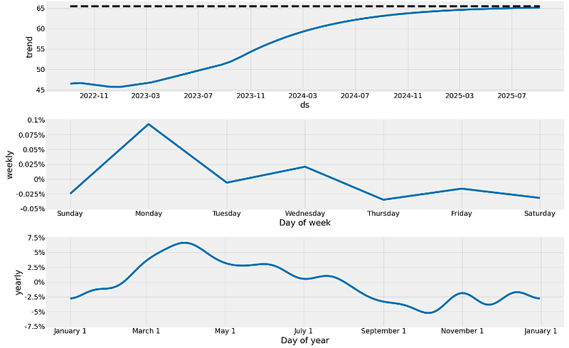
- Plotting the forecast vs actual values of BTC-USD prices
model.plot(forecast,figsize=(14, 8));# block dots are actual values and blue dots are forecast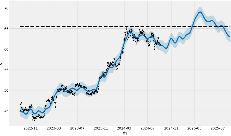
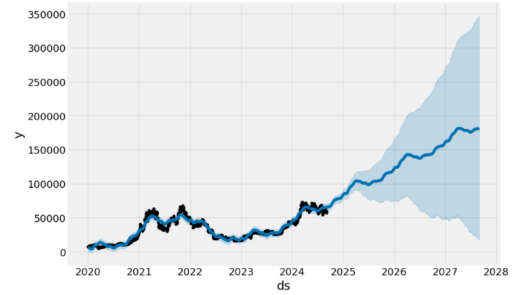
- Here, the dashed line indicates a cap or upper limit for the forecast.
- We should remember that the out-of-sample forecast was built using all of the data prior to the forecast period. As an example, the forecast for 2025 was built using using data up to and including September 4, 2024.
- Adding the monthly/quarterly seasonality and US events
## Adding parameters and seasonality and events
model = Prophet(**model_param)

model= model.add_seasonality(name="monthly", period=30, fourier_order=10)
model= model.add_seasonality(name="quarterly", period=92.25, fourier_order=10)

model.add_country_holidays("US")

model.fit(data1)

# Create future dataframe
future= model.make_future_dataframe(periods=365)
future['cap'] = data1['cap'].max()

forecast= model.predict(future)

from prophet.plot import plot

plot(model, forecast, figsize=(14, 8))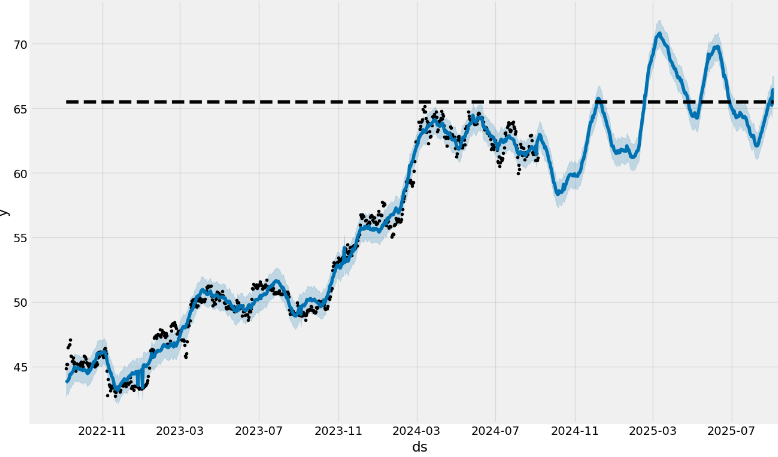
- Notice a somewhat increased frequency content and a narrow confidence interval (CI) of the above out-of-sample predictions as compared to the forecast without monthly/quarterly seasonality and US events.
- Plotting the Prophet trend, US holidays, and seasonality
from prophet.plot import plot_components

plot_components(model, forecast, figsize=(12, 12))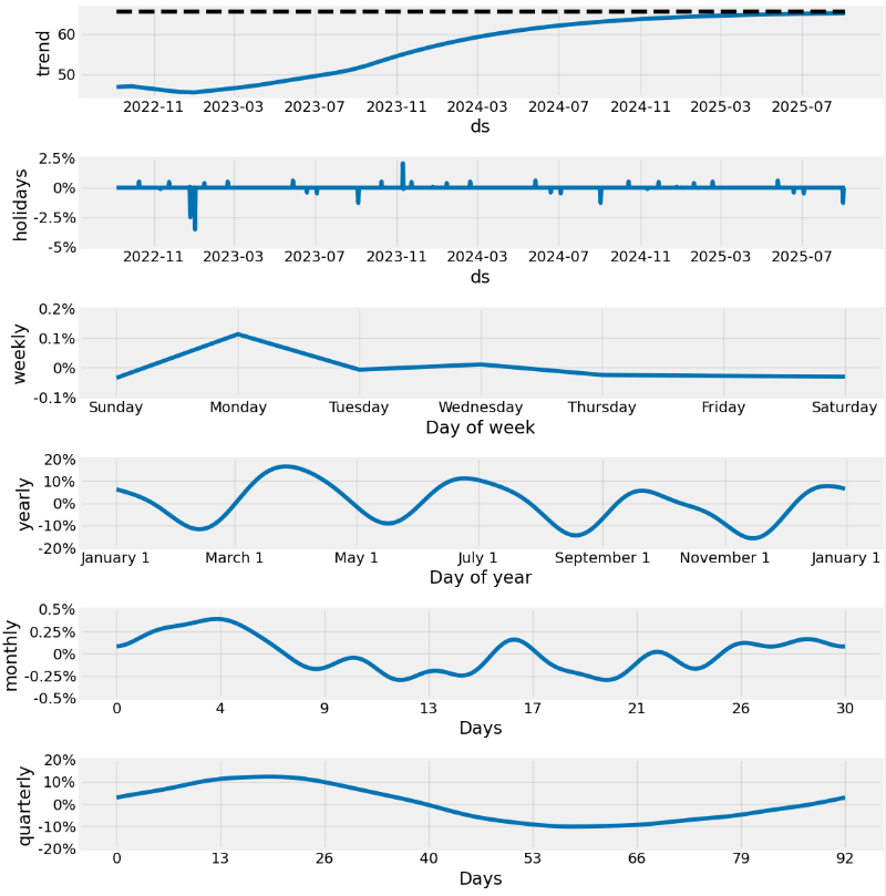
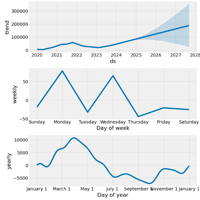
We see a few features in the above components:
- A strong upward trend with a change in the rate of increase somewhere between 2023–11 and 2024–06
- Fairly strong yearly seasonality
- Variable monthly seasonal effect.
The generated forecast will have many columns as shown in the below output. We will go over the significant ones:
- yhat: This column has the predictions for the number of transactions for the future timestamps.
- yhat_lower: Prophet also takes into account the uncertainty levels while making predictions. This represents the lower bound of the uncertainty interval for each forecasted value.
- yhat_upper: This column represents the upper bound of the uncertainty interval for each forecasted value.
- trend: This represents the estimated trend component of the forecast, the overall direction of growth.
Performing a reverse Box-Cox transformation and plotting yhat, yhat_lower, and yhat_upper
forecast["yhat"]=bc.untransform_boxcox(x=forecast["yhat"], lmbda=lmbda)
forecast["yhat_lower"]=bc.untransform_boxcox(x=forecast["yhat_lower"], lmbda=lmbda)
forecast["yhat_upper"]=bc.untransform_boxcox(x=forecast["yhat_upper"], lmbda=lmbda)
forecast.plot(x="ds", y=["yhat_lower", "yhat", "yhat_upper"])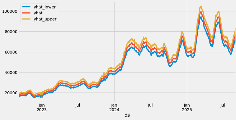
- Examining the Prophet cross-validation metrics with horizon=’90 days’
from prophet.diagnostics import cross_validation, performance_metrics
from prophet.plot import plot_cross_validation_metric
df_cv = cross_validation(model, initial="600 days", period="30 days", horizon="90 days")
cutoffs = pd.to_datetime(['2022-09-01', '2023-05-01', '2024-03-01'])
df_cv2 = cross_validation(model, cutoffs=cutoffs, horizon='90 days')
fig = plot_cross_validation_metric(df_cv2, metric='mae')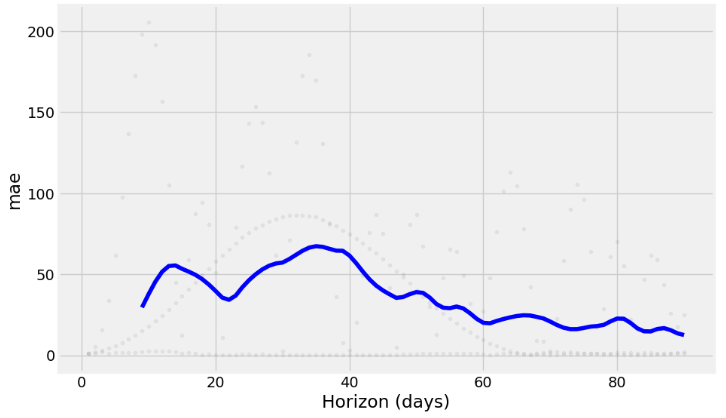
- One cool feature is that we can see the error metric per day.
- Performing the Prophet hyperparameter optimization (HPO) [12]
## Hyper parameter Tuning
import itertools
import numpy as np
from prophet.diagnostics import cross_validation, performance_metrics


param_grid={
    "daily_seasonality": [False],
    "weekly_seasonality":[True],
    "yearly_seasonality":[True],
    "growth": ["logistic"],
    'changepoint_prior_scale': [0.001, 0.01, 0.1, 0.5], # to give higher value to prior trend
    'seasonality_prior_scale': [0.01, 0.1, 1.0, 10.0] # to control the flexibility of seasonality components
}

# Generate all combination of parameters
all_params= [
            dict(zip(param_grid.keys(), v))
            for v in itertools.product(*param_grid.values())
]

rmses= list ()

# go through each combinations
for params in all_params:
    m= Prophet(**params)

    m= m.add_seasonality(name= 'monthly', period=30, fourier_order=5)
    m= m.add_seasonality(name= "quarterly", period= 92.25, fourier_order= 10)


    m.add_country_holidays(country_name="US")

    m.fit(data1)

    df_cv= cross_validation(m, initial="500 days", period="180 days", horizon="90 days")

    df_p= performance_metrics(df_cv, rolling_window=1)

    rmses.append(df_p['rmse'].values[0])

# find teh best parameters
best_params = all_params[np.argmin(rmses)]

print("\n The best parameters are:", best_params)

The best parameters are: {'daily_seasonality': False, 'weekly_seasonality': True, 'yearly_seasonality': True, 'growth': 'logistic', 'changepoint_prior_scale': 0.001, 'seasonality_prior_scale': 0.01}- After HPO: performing a reverse Box-Cox transformation and plotting yhat, yhat_lower, and yhat_upper
forecast["yhat"]=bc.untransform_boxcox(x=forecast["yhat"], lmbda=lmbda)
forecast["yhat_lower"]=bc.untransform_boxcox(x=forecast["yhat_lower"], lmbda=lmbda)
forecast["yhat_upper"]=bc.untransform_boxcox(x=forecast["yhat_upper"], lmbda=lmbda)
forecast.plot(x="ds", y=["yhat_lower", "yhat", "yhat_upper"])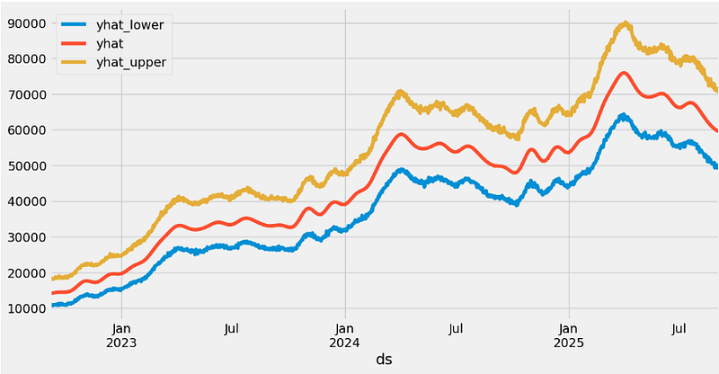
- Running the cross-validation and use a range of built-in metrics to evaluate the performance of our model, such as mean absolute error (MAE), mean squared error (MSE), mean average percentage error (MAPE), or root mean squared error (RMSE) with horizon=’180 days’, viz.
df_cv2 = cross_validation(model1, horizon='180 days')
fig = plot_cross_validation_metric(df_cv2, metric='rmse')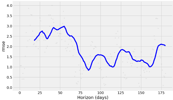
fig = plot_cross_validation_metric(df_cv2, metric='mape')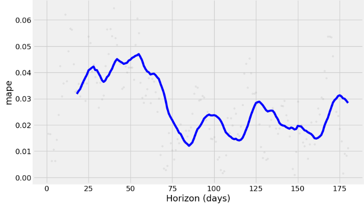
fig = plot_cross_validation_metric(df_cv2, metric='mae')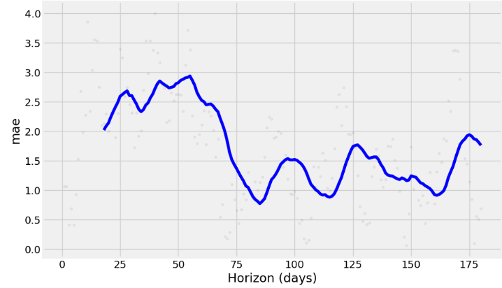
- The charts above show how reliable the forecast is over a specific time horizon. The above built-in metrics give us a good enough estimation of the model’s performance.
2020–2027 Time Horizon
- Next, let’s create a 3 year Prophet forecast [13] until 2027–09–03 using the historical daily BTC-USD adjusted close price data from 2020–01–01 to 2024–09–05.
- Reading the input BTC-USD stock data and preparing a dataframe with two columns — ds and y
import pandas as pd
import numpy as np
from prophet import Prophet
import matplotlib.pyplot as plt
from functools import reduce

%matplotlib inline
import warnings
warnings.filterwarnings('ignore')

pd.options.display.float_format = "{:,.2f}".format

import yfinance as yf

ticker = 'BTC-USD'
start_date = '2020-01-01'

stock_price = yf.download(ticker, start=start_date)
stock_price["Date"] = stock_price.index
stock_price.tail()

           Open      High      Low       Close     Adj Close Volume       Date
Date
2024-09-01 58,969.80 59,062.07 57,217.82 57,325.49 57,325.49 24592449997 2024-09-01
2024-09-02 57,326.97 59,403.07 57,136.03 59,112.48 59,112.48 27036454524 2024-09-02
2024-09-03 59,106.19 59,815.06 57,425.17 57,431.02 57,431.02 26666961053 2024-09-03
2024-09-04 57,430.35 58,511.57 55,673.16 57,971.54 57,971.54 35627680312 2024-09-04
2024-09-05 57,969.75 58,280.16 56,441.49 56,816.75 56,816.75 31623784448 2024-09-05


stock_price = stock_price[['Date','Adj Close']]

stock_price.columns = ['ds', 'y']
stock_price.tail()

           ds          y
Date
2024-09-01 2024-09-01 57,325.49
2024-09-02 2024-09-02 59,112.48
2024-09-03 2024-09-03 57,431.02
2024-09-04 2024-09-04 57,971.54
2024-09-05 2024-09-05 56,816.75- Fitting the above stock price and making predictions for future dates
model = Prophet()
model.fit(stock_price)

future = model.make_future_dataframe(1095, freq='d')

future_boolean = future['ds'].map(lambda x : True if x.weekday() in range(0, 5) else False)
future = future[future_boolean]

future.tail()

ds
2798 2027-08-30
2799 2027-08-31
2800 2027-09-01
2801 2027-09-02
2802 2027-09-03

forecast = model.predict(future)
forecast.tail()

      ds        trend      yhat_lower yhat_upper trend_lower trend_upper additive_terms additive_terms_lower additive_terms_upper weekly weekly_lower weekly_upper yearly yearly_lower yearly_upper multiplicative_terms multiplicative_terms_lower multiplicative_terms_upper yhat
1998 2027-08-30 186,397.72 17,078.78 342,504.45 25,330.76 349,736.48 -5,418.98 -5,418.98 -5,418.98 77.78 77.78 77.78 -5,496.76 -5,496.76 -5,496.76 0.00 0.00 0.00 180,978.73
1999 2027-08-31 186,503.42 18,938.28 343,364.67 25,153.02 350,048.12 -5,602.41 -5,602.41 -5,602.41 -32.66 -32.66 -32.66 -5,569.75 -5,569.75 -5,569.75 0.00 0.00 0.00 180,901.01
2000 2027-09-01 186,609.12 16,790.94 346,802.89 24,995.28 350,535.01 -5,574.97 -5,574.97 -5,574.97 64.88 64.88 64.88 -5,639.84 -5,639.84 -5,639.84 0.00 0.00 0.00 181,034.16
2001 2027-09-02 186,714.83 20,909.35 347,787.00 24,837.54 351,021.90 -5,751.63 -5,751.63 -5,751.63 -44.32 -44.32 -44.32 -5,707.31 -5,707.31 -5,707.31 0.00 0.00 0.00 180,963.20
2002 2027-09-03 186,820.53 18,715.76 344,767.13 24,487.82 351,508.79 -5,793.51 -5,793.51 -5,793.51 -21.00 -21.00 -21.00 -5,772.52 -5,772.52 -5,772.52 0.00 0.00 0.00 181,027.02- Plotting the 3Y forecast with CI
model.plot(forecast);
- Plotting the key components: trend and seasonality
model.plot_components(forecast);
- Plotting the 3Y forecast in terms of yhat, yhat_lower, and yhat_upper
stock_price_forecast = forecast[['ds', 'yhat', 'yhat_lower', 'yhat_upper']]
df = pd.merge(stock_price, stock_price_forecast, on='ds', how='right')
df.set_index('ds').plot(figsize=(16,8), color=['royalblue', "#34495e", "#e74c3c", "#e74c3c"], grid=True);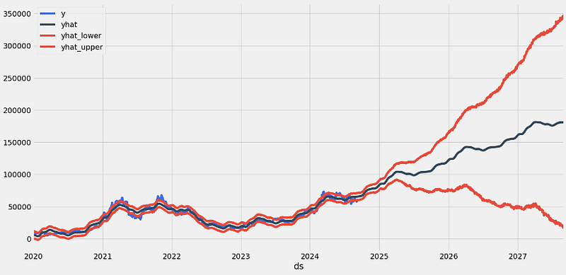
- Splitting the date index [13] and making the Prophet forecast
stock_price['dayname'] = stock_price['ds'].dt.day_name()
stock_price['month'] = stock_price['ds'].dt.month
stock_price['year'] = stock_price['ds'].dt.year
stock_price['month/year'] = stock_price['month'].map(str) + '/' + stock_price['year'].map(str)

stock_price = pd.merge(stock_price,
                       stock_price['month/year'].drop_duplicates().reset_index(drop=True).reset_index(),
                       on='month/year',
                       how='left')

stock_price = stock_price.rename(columns={'index':'month/year_index'})

loop_list = stock_price['month/year'].unique().tolist()
max_num = len(loop_list) - 1
forecast_frames = []

for num, item in enumerate(loop_list):

    if  num == max_num:
        pass
    else:
        df = stock_price.set_index('ds')[
             stock_price[stock_price['month/year'] == loop_list[0]]['ds'].min():\
             stock_price[stock_price['month/year'] == item]['ds'].max()]

        df = df.reset_index()[['ds', 'y']]

        model = Prophet()
        model.fit(df)

        future = stock_price[stock_price['month/year_index'] == (num + 1)][['ds']]

        forecast = model.predict(future)
        forecast_frames.append(forecast)

stock_price_forecast = reduce(lambda top, bottom: pd.concat([top, bottom], sort=False), forecast_frames)
stock_price_forecast = stock_price_forecast[['ds', 'yhat', 'yhat_lower', 'yhat_upper']]

df = pd.merge(stock_price[['ds','y', 'month/year_index']], stock_price_forecast, on='ds')
df['Percent Change'] = df['y'].pct_change()
df.set_index('ds')[['y', 'yhat', 'yhat_lower', 'yhat_upper']].plot(figsize=(16,8), color=['royalblue', "#34495e", "#e74c3c", "#e74c3c"], grid=True)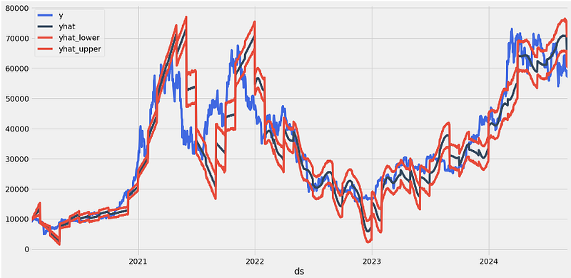
- Running the Prophet cross-validation QC diagnostics
from prophet.diagnostics import cross_validation
df_cv = cross_validation(model, initial='600 days', period='180 days', horizon = '365 days')

from prophet.diagnostics import performance_metrics
df_p = performance_metrics(df_cv)
df_p.head()

  horizon mse           rmse     mae      mape mdape smape coverage
0 37 days 37,926,228.96 6,158.43 5,078.86 0.16 0.14 0.17 0.41
1 38 days 39,286,966.57 6,267.93 5,205.29 0.16 0.14 0.17 0.40
2 39 days 40,986,172.18 6,402.04 5,344.08 0.16 0.15 0.18 0.39
3 40 days 42,315,522.99 6,505.04 5,454.70 0.17 0.15 0.18 0.38
4 41 days 43,420,106.74 6,589.39 5,544.55 0.17 0.15 0.18 0.37

from prophet.plot import plot_cross_validation_metric
fig = plot_cross_validation_metric(df_cv, metric='rmse')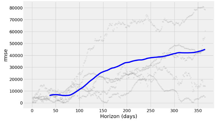
fig = plot_cross_validation_metric(df_cv, metric='mape')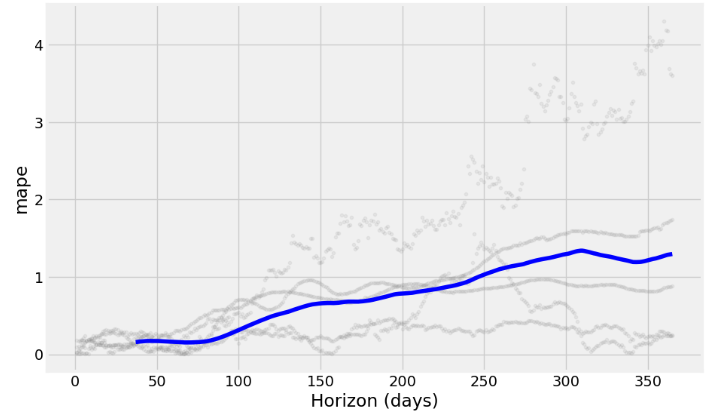
fig = plot_cross_validation_metric(df_cv, metric='mae')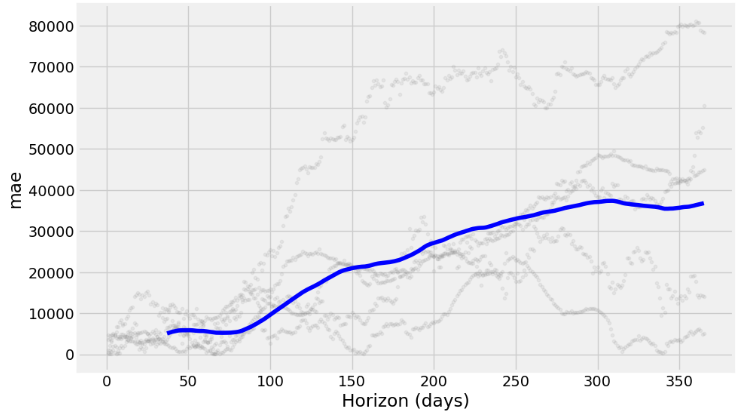
- Running HPO [17] by defining the hyperparameter grid
from sklearn.metrics import mean_absolute_error
param_grid = {
    'seasonality_mode': ['additive', 'multiplicative'],
    'changepoint_prior_scale': [0.01, 0.1, 1, 10],
    'seasonality_prior_scale': [0.01, 0.1, 1, 10],
}


# Helper function to evaluate the model
def evaluate_model(model, metric_func):
    df_cv = cross_validation(model, initial='1125 days', period='180 days', horizon='365 days')
    return metric_func(df_cv['y'], df_cv['yhat'])


# Grid search
best_params = {}
best_score = float('inf')

for mode in param_grid['seasonality_mode']:
    for cps in param_grid['changepoint_prior_scale']:
        for sps in param_grid['seasonality_prior_scale']:
            # Create a model with the current hyperparameters
            m = Prophet(seasonality_mode=mode, changepoint_prior_scale=cps, seasonality_prior_scale=sps)
            m.fit(stock_price)

            # Evaluate the model using Mean Absolute Error (MAE)
            score = evaluate_model(m, mean_absolute_error)

            # Update best parameters if necessary
            if score < best_score:
                best_score = score
                best_params = {
                    'seasonality_mode': mode,
                    'changepoint_prior_scale': cps,
                    'seasonality_prior_scale': sps
                }

print(best_params)
print(best_score)

{'seasonality_mode': 'multiplicative', 'changepoint_prior_scale': 1, 'seasonality_prior_scale': 0.01}
13078.117877655675- Defining the HPO-updated Prophet model and making 1Y predictions
#Model with best parameters
m_best = Prophet(seasonality_mode= 'additive', changepoint_prior_scale = 1, seasonality_prior_scale = 0.01)
m_best.fit(stock_price)

#dataframe for the forecast(with 365 days)
future_best = m_best.make_future_dataframe(periods=365)
forecast_best = m_best.predict(future_best)

#plot the graph with the forecast data
fig1 = m.plot(forecast_best)
ax = fig1.gca()
ax.set_title("BTC-USD Stock Price Forecast", size=25)
ax.set_xlabel("Date", size=15)
ax.set_ylabel("Price", size=15)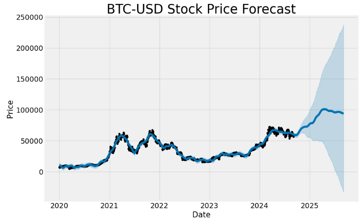
- Performing cross-validation QC
# Perform cross-validation
from sklearn.metrics import mean_squared_error
df_cv = cross_validation(m_best, initial='1125 days', period='180 days', horizon='365 days')

# Calculate performance metrics
df_metrics = performance_metrics(df_cv)

# Calculate MAE, MSE, and RMSE
mae = mean_absolute_error(df_cv['y'], df_cv['yhat'])
mse = mean_squared_error(df_cv['y'], df_cv['yhat'])
rmse = np.sqrt(mse)

print(f'Mean Absolute Error: {mae:.2f}')
print(f'Mean Squared Error: {mse:.2f}')
print(f'Root Mean Squared Error: {rmse:.2f}')

Mean Absolute Error: 13879.24
Mean Squared Error: 279497823.66
Root Mean Squared Error: 16718.19- Plotting RMSE, MAPE, and MAE vs Horizon (days)
from prophet.plot import plot_cross_validation_metric
df_cv = cross_validation(m_best, initial='1125 days', period='180 days', horizon='365 days')
fig = plot_cross_validation_metric(df_cv, metric='rmse')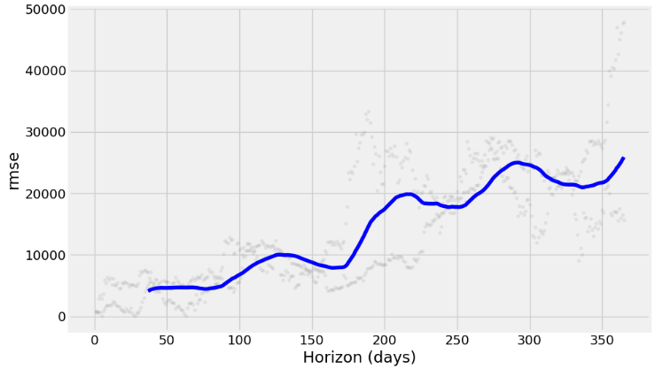
fig = plot_cross_validation_metric(df_cv, metric='mape')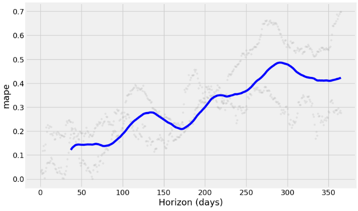
fig = plot_cross_validation_metric(df_cv, metric='mae')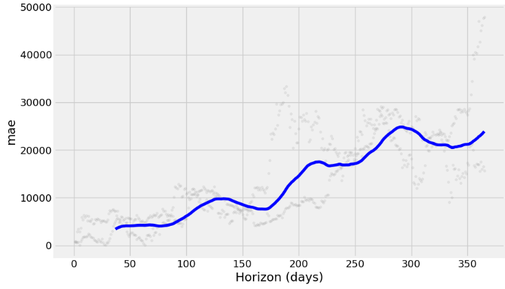
- Splitting the date index [13] and making the Prophet in-sample forecast
loop_list = stock_price['month/year'].unique().tolist()
max_num = len(loop_list) - 1
forecast_frames = []

for num, item in enumerate(loop_list):

    if  num == max_num:
        pass
    else:
        df = stock_price.set_index('ds')[
             stock_price[stock_price['month/year'] == loop_list[0]]['ds'].min():\
             stock_price[stock_price['month/year'] == item]['ds'].max()]

        df = df.reset_index()[['ds', 'y']]

        future = stock_price[stock_price['month/year_index'] == (num + 1)][['ds']]

        forecast = m_best.predict(future)
        forecast_frames.append(forecast)

stock_price_forecast1 = reduce(lambda top, bottom: pd.concat([top, bottom], sort=False), forecast_frames)
stock_price_forecast1 = stock_price_forecast1[['ds', 'yhat', 'yhat_lower', 'yhat_upper']]

df1 = pd.merge(stock_price[['ds','y', 'month/year_index']], stock_price_forecast1, on='ds')
df1['Percent Change'] = df1['y'].pct_change()
df1.set_index('ds')[['y', 'yhat', 'yhat_lower', 'yhat_upper']].plot(figsize=(16,8), color=['royalblue', "#34495e", "#e74c3c", "#e74c3c"], grid=True)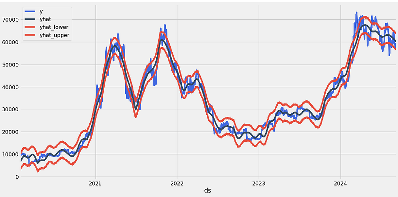
Prophet Algo-Trading Strategies [13]
- Backtesting the BTC-USD HPO-updated Prophet algo-trading strategy
#Trading Algorithms
df=df1.copy()
df['Hold'] = (df['Percent Change'] + 1).cumprod()
df['Prophet'] = ((df['yhat'].shift(-1) > df['yhat']).shift(1) * (df['Percent Change']) + 1).cumprod()
df['Prophet Thresh']  = ((df['y'] < df['yhat_upper']).shift(1)* (df['Percent Change']) + 1).cumprod()
df['Seasonality'] = ((~df['ds'].dt.month.isin([8,9])).shift(1) * (df['Percent Change']) + 1).cumprod()

(df.dropna().set_index('ds')[['Hold', 'Prophet', 'Prophet Thresh','Seasonality']] * 1000).plot(figsize=(16,8), grid=True)

print(f"Hold = {df['Hold'].iloc[-1]*1000:,.0f}")
print(f"Prophet = {df['Prophet'].iloc[-1]*1000:,.0f}")
print(f"Prophet Thresh = {df['Prophet Thresh'].iloc[-1]*1000:,.0f}")
print(f"Seasonality = {df['Seasonality'].iloc[-1]*1000:,.0f}")

Hold = 6,049
Prophet = 62,849
Prophet Thresh = 23,986
Seasonality = 8,195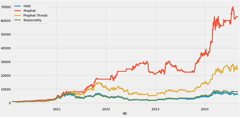
- Optimizing the Prophet threshold value in the range 0.9–1.0
performance = {}

for x in np.linspace(.9,.99,10):
    y = ((df['y'] < df['yhat_upper']*x).shift(1)* (df['Percent Change']) + 1).cumprod()
    performance[x] = y

best_yhat = pd.DataFrame(performance).max().idxmax()
pd.DataFrame(performance).plot(figsize=(16,8), grid=True);
f'Best Yhat = {best_yhat:,.2f}'

'Best Yhat = 0.90'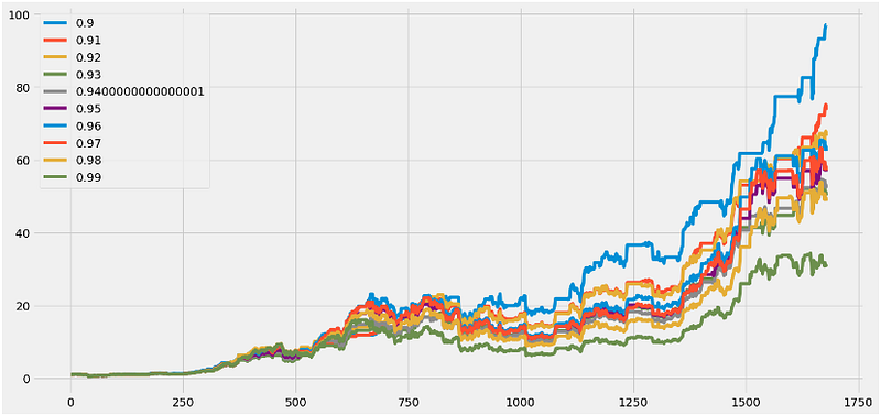
- Backtesting the BTC-USD HPO-updated Prophet algo-trading strategy with the optimized threshold value Best Yhat = 0.90
df['Optimized Prophet Thresh']  = ((df['y'] < df['yhat_upper'] * best_yhat).shift(1) *
                                   (df['Percent Change']) + 1).cumprod()

(df.dropna().set_index('ds')[['Hold', 'Prophet', 'Prophet Thresh',
                              'Seasonality', 'Optimized Prophet Thresh']] * 1000).plot(figsize=(16,8), grid=True)

print(f"Hold = {df['Hold'].iloc[-1]*1000:,.0f}")
print(f"Prophet = {df['Prophet'].iloc[-1]*1000:,.0f}")
print(f"Prophet Thresh = {df['Prophet Thresh'].iloc[-1]*1000:,.0f}")
print(f"Seasonality = {df['Seasonality'].iloc[-1]*1000:,.0f}")
print(f"Optimized Prophet Thresh = {df['Optimized Prophet Thresh'].iloc[-1]*1000:,.0f}")

Hold = 6,049
Prophet = 62,849
Prophet Thresh = 23,986
Seasonality = 8,195
Optimized Prophet Thresh = 97,000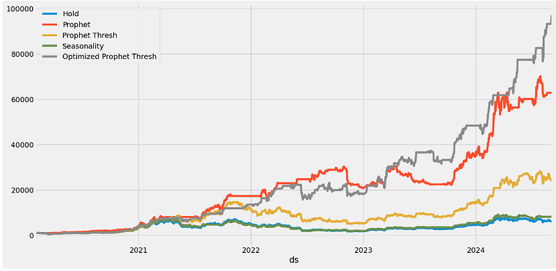
Prophet Plotly with Changepoints
- Making 1Y Prophet predictions with changepoints and Plotly visuals
stock_price.tail()

     ds         y       dayname month year month/year month/year_index
1705 2024-09-01 57,325.49 Sunday 9 2024 9/2024 56
1706 2024-09-02 59,112.48 Monday 9 2024 9/2024 56
1707 2024-09-03 57,431.02 Tuesday 9 2024 9/2024 56
1708 2024-09-04 57,971.54 Wednesday 9 2024 9/2024 56
1709 2024-09-05 56,816.75 Thursday 9 2024 9/2024 56

mydf=stock_price[['ds','y']]

mm = Prophet()
mm.fit(mydf)

future = mm.make_future_dataframe(periods=365)

forecast = mm.predict(future)

from prophet.plot import plot_plotly

plot_plotly(mm, forecast)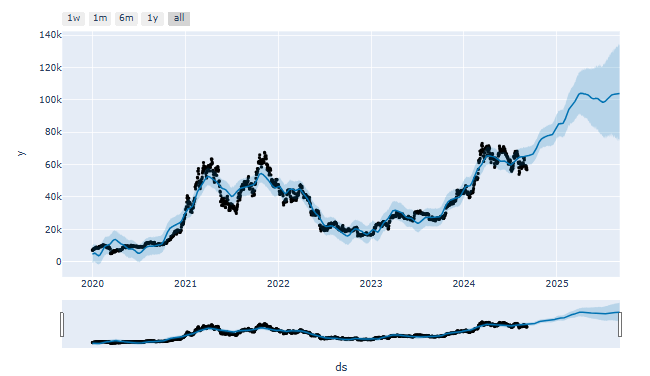
- Plotting Prophet predictions with changepoints in Plotly
from prophet.plot import plot_plotly

plot_plotly(mm, forecast, changepoints=True)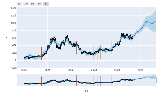
- Plotting Prophet 1Y forecast: key components in Plotly
from prophet.plot import plot_components_plotly

### Using plotly
plot_components_plotly(m, forecast)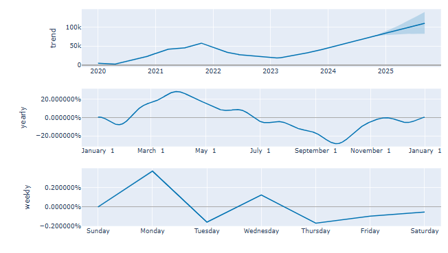
- Running cross-validation QC
from prophet.diagnostics import cross_validation

df_cv = cross_validation(mm, initial='540 days', period='31 days', horizon = '180 days')

from prophet.diagnostics import performance_metrics
df_p = performance_metrics(df_cv)
df_p.head(2)

horizon   mse           rmse      mae     mape mdape smape coverage
0 18 days 48,591,983.30 6,970.80 5,096.63 0.15 0.12 0.16 0.52
1 19 days 51,427,421.78 7,171.29 5,260.73 0.15 0.12 0.16 0.50- Plotting MAPE vs Horizon (days)
from prophet.plot import plot_cross_validation_metric

fig = plot_cross_validation_metric(df_cv, metric='mape')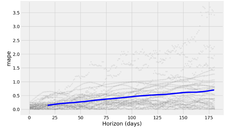
- Plotting MAE vs Horizon (days)
fig = plot_cross_validation_metric(df_cv, metric='mae')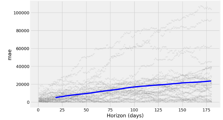
- Plotting RMSE vs Horizon (days)
fig = plot_cross_validation_metric(df_cv, metric='rmse')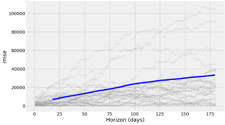
Inferences:
- Prophet with the Box-Cox transformation and a cap or upper limit for the forecast yields the 1Y prediction with relatively narrow CI and can capture non-linearity in the trend of the data
- Adding the monthly/quarterly seasonality and US events reveals a fairly strong yearly seasonality and a somewhat increased frequency content with reasonable CI of the out-of-sample predictions.
- 1Y forecast (2022–2027 time interval): combining the Box-Cox transformation and HPO reduces MAE about 20 times.
- 2020–2027 Time Interval: Splitting the date index improves the in-sample goodness-of-fit of the Prophet forecast.
- The HPO-updated Prophet model and 1Y predictions yield
Mean Absolute Error: 13879.24
Mean Squared Error: 279497823.66
Root Mean Squared Error: 16718.19- Backtesting of algo-trading strategies result in the following expected returns
Hold = 6,049
Prophet = 62,849
Prophet Thresh = 23,986
Seasonality = 8,195
Optimized Prophet Thresh = 97,000- Prophet provides an interpretable decomposition of the data that is observed or forecasted into trend and multi-seasonal components.
- Different useful plotting options are available in Prophet: forecasts in terms of yhat/yhat_lower/yhat_upper, cross-validation metrics, Plotly plots with changepoints, etc.
NVDA Price Prediction using Auto-ARIMA, Supervised ML & Technical Indicators
- It is well known that ML can be used to forecast stock values in the future or find lucrative trading opportunities on the stock market [25].
- This section aims to design, train, and evaluate ML-powered NVDA price prediction algorithms in the context of quantitative finance.
- Specifically, our objective is to demonstrate how Auto-ARIMA and popular supervised ML algorithms with technical indicators [18, 19] can add value to algorithmic trading strategies in a practical yet comprehensive way.
NVDA EDA
- Setting the working directory YOURPATH
import os
os.chdir('YOURPATH')    # Set working directory
os. getcwd() - Importing the necessary Python libraries
#Import Libraries
import pandas as pd
import numpy as np

import matplotlib.pyplot as plt
import seaborn as sns
sns.set_style('whitegrid')
plt.style.use("fivethirtyeight")
%matplotlib inline

# For reading stock data from yahoo


import yfinance as yf

# For time stamps
from datetime import datetime
from math import sqrt
from math import sqrt
from sklearn.metrics import mean_squared_error
from sklearn.preprocessing import MinMaxScaler

#ignore the warnings
import warnings
warnings.filterwarnings('ignore')- Reading the input stock data from 2020–01–01 to 2024–09–06
symbols = ['NVDA']
start_date = '2020-01-01'

data = yf.download(symbols, start=start_date)
data.tail()

           Open       High       Low        Close      Adj Close   Volume
Date
2024-08-30 119.529999 121.750000 117.220001 119.370003 119.370003 333751600
2024-09-03 116.010002 116.209999 107.290001 108.000000 108.000000 474040800
2024-09-04 105.410004 113.269997 104.120003 106.209999 106.209999 372470300
2024-09-05 104.989998 109.650002 104.760002 107.209999 107.209999 306850700
2024-09-06 108.040001 108.150002 100.949997 102.830002 102.830002 411712100- Plotting the Close price history
def plot_close_val(data_frame, column, stock):
    plt.figure(figsize=(10,6))
    plt.title(column + ' Price History for ' + stock )
    plt.plot(data_frame[column])
    plt.xlabel('Date', fontsize=18)
    plt.ylabel(column + ' Price USD ($) for ' + stock, fontsize=18)
    plt.show()

#Test the function
plot_close_val(data, 'Close', 'NVDA')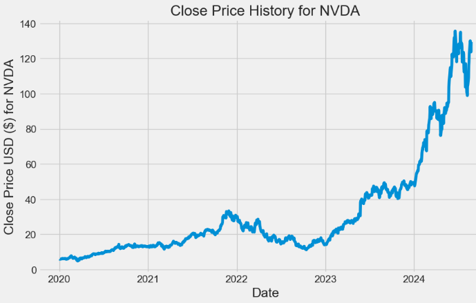
- Plotting the histogram of daily returns
#Basic EDA
daily_close_px = data[['Close']]
# Calculate the daily percentage change for `daily_close_px`
daily_pct_change = daily_close_px.pct_change()

# Plot the distributions
daily_pct_change.hist(bins=50, sharex=True, figsize=(12,8))

# Show the resulting plot
plt.show()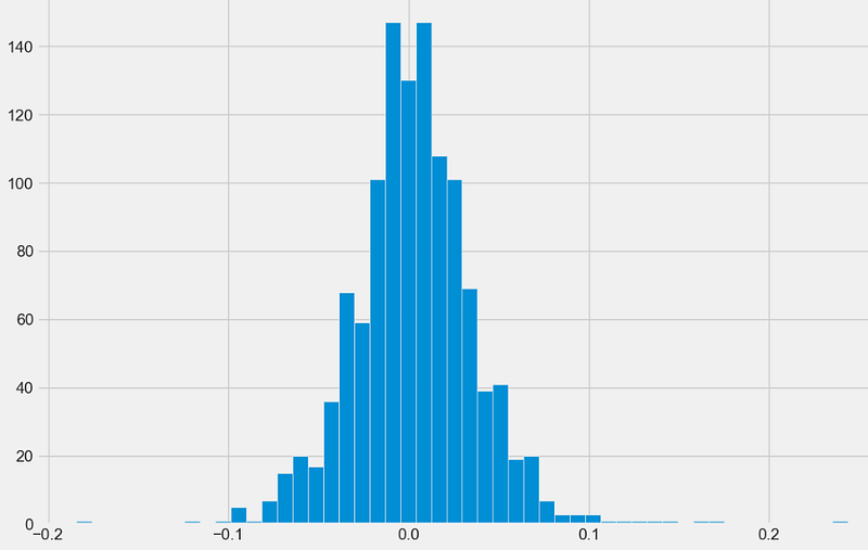
- Plotting the rolling STD of Close price with min_periods = 75
# Define the minumum of periods to consider
min_periods = 75

# Calculate the volatility
vol = daily_pct_change.rolling(min_periods).std() * np.sqrt(min_periods)

# Plot the volatility
vol.plot(figsize=(10, 6))

# Show the plot
plt.show()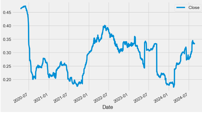
- Plotting the NVDA candlestick chart
import plotly.graph_objects as go

data=data.reset_index()

fig = go.Figure(data=go.Ohlc(x=data['Date'],
        open=data['Open'],
        high=data['High'],
        low=data['Low'],
        close=data['Close']))
fig.show()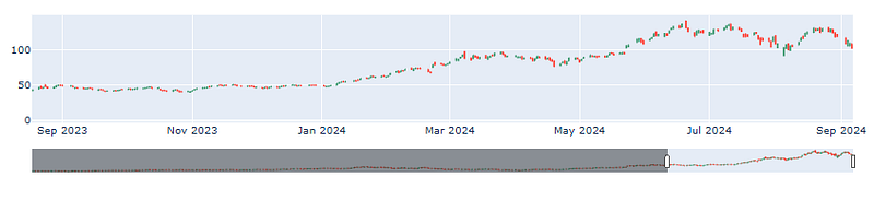
- Plotting the NVDA candlestick chart with top 5 simple moving averages (SMA 5, 20, 50, 200, 500)
data=data.reset_index()

data['SMA5'] = data.Close.rolling(5).mean()
data['SMA20'] = data.Close.rolling(20).mean()
data['SMA50'] = data.Close.rolling(50).mean()
data['SMA200'] = data.Close.rolling(200).mean()
data['SMA500'] = data.Close.rolling(500).mean()

fig = go.Figure(data=[go.Ohlc(x=data['Date'],open=data['Open'],high=data['High'],low=data['Low'],close=data['Close'], name = "OHLC"),
                      go.Scatter(x=data.Date, y=data.SMA5, line=dict(color='orange', width=1), name="SMA5"),
                      go.Scatter(x=data.Date, y=data.SMA20, line=dict(color='green', width=1), name="SMA20"),
                      go.Scatter(x=data.Date, y=data.SMA50, line=dict(color='blue', width=1), name="SMA50"),
                      go.Scatter(x=data.Date, y=data.SMA200, line=dict(color='violet', width=1), name="SMA200"),
                      go.Scatter(x=data.Date, y=data.SMA500, line=dict(color='purple', width=1), name="SMA500")])
fig.show()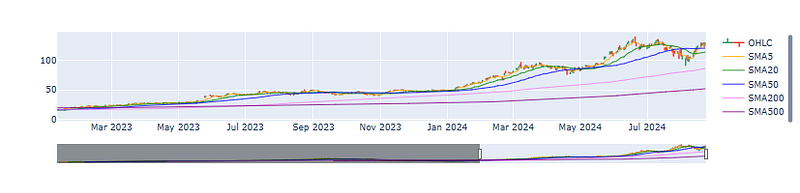
Auto-ARIMA Modeling [18]
- Preparing the W-MON resampled Open price for statistical modeling
x = data['Open'].resample('W-MON').mean()
x.head()

Date
2020-01-06    5.884750
2020-01-13    6.084000
2020-01-20    6.221687
2020-01-27    6.225150
2020-02-03    6.057600
Freq: W-MON, Name: Open, dtype: float64

#visualize time series of open price
x.plot(figsize = (10,6))
plt.title("Opening Price")
plt.show()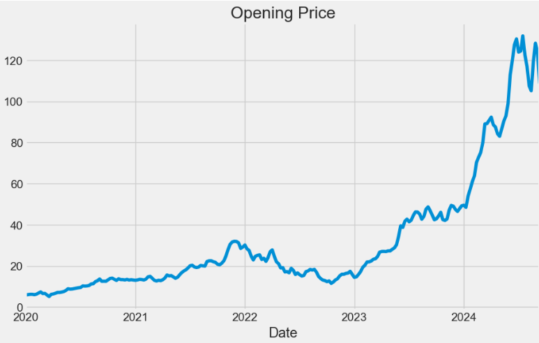
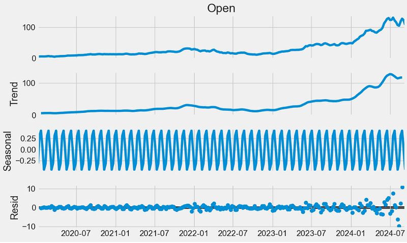
- Using statsmodels to perform the additive trend-seasonality decomposition
- Plotting the autocorrelation function
from pandas.plotting import autocorrelation_plot
from statsmodels.tsa.stattools import adfuller, kpss
plt.rcParams.update({'figure.figsize':(10,6), 'figure.dpi':120})
autocorrelation_plot(x.tolist())
plt.grid(color='grey')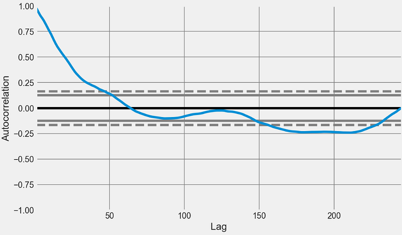
- Finding an optimal parameter combination for Seasonal ARIMA without enforcing stationarity of time series
import warnings
import itertools

p = d = q = range(0, 2)
pdq = list(itertools.product(p, d, q))
seasonal_pdq = [(x[0], x[1], x[2], 12) for x in list(itertools.product(p, d, q))]
print('Examples of parameter combinations for Seasonal ARIMA...')
print('SARIMAX: {} x {}'.format(pdq[1], seasonal_pdq[1]))
print('SARIMAX: {} x {}'.format(pdq[1], seasonal_pdq[2]))
print('SARIMAX: {} x {}'.format(pdq[2], seasonal_pdq[3]))
print('SARIMAX: {} x {}'.format(pdq[2], seasonal_pdq[4]))

Examples of parameter combinations for Seasonal ARIMA...
SARIMAX: (0, 0, 1) x (0, 0, 1, 12)
SARIMAX: (0, 0, 1) x (0, 1, 0, 12)
SARIMAX: (0, 1, 0) x (0, 1, 1, 12)
SARIMAX: (0, 1, 0) x (1, 0, 0, 12)

#selection of parameter
for param in pdq:
    for param_seasonal in seasonal_pdq:
        try:
            model = sm.tsa.statespace.SARIMAX(x, order = param, seasonal_order = param_seasonal, enforce_stationarity = False,
                                            enforce_invertibility = False)
            results = model.fit()
            print('ARIMA{}x{}12 - AIC:{}'.format(param, param_seasonal, results.aic))
        except:
                continue

ARIMA(0, 0, 0)x(0, 0, 0, 12)12 - AIC:2542.1221453228754
ARIMA(0, 0, 0)x(0, 0, 1, 12)12 - AIC:2205.432369780864
ARIMA(0, 0, 0)x(0, 1, 0, 12)12 - AIC:1826.8913110661877
ARIMA(0, 0, 0)x(0, 1, 1, 12)12 - AIC:1663.0856888581307
ARIMA(0, 0, 0)x(1, 0, 0, 12)12 - AIC:1696.5162260417578
ARIMA(0, 0, 0)x(1, 0, 1, 12)12 - AIC:1678.9637064852432
ARIMA(0, 0, 0)x(1, 1, 0, 12)12 - AIC:1651.058267917132
ARIMA(0, 0, 0)x(1, 1, 1, 12)12 - AIC:1645.9164183133007
ARIMA(0, 0, 1)x(0, 0, 0, 12)12 - AIC:2210.7423692662937
ARIMA(0, 0, 1)x(0, 0, 1, 12)12 - AIC:2203.0913037562423
ARIMA(0, 0, 1)x(0, 1, 0, 12)12 - AIC:1537.3048930586983
ARIMA(0, 0, 1)x(0, 1, 1, 12)12 - AIC:1418.7522928794192
ARIMA(0, 0, 1)x(1, 0, 0, 12)12 - AIC:1451.0683837824945
ARIMA(0, 0, 1)x(1, 0, 1, 12)12 - AIC:1441.0113195138251
ARIMA(0, 0, 1)x(1, 1, 0, 12)12 - AIC:1423.0785411142224
ARIMA(0, 0, 1)x(1, 1, 1, 12)12 - AIC:1413.039982679135
ARIMA(0, 1, 0)x(0, 0, 0, 12)12 - AIC:1178.8567047336762
ARIMA(0, 1, 0)x(0, 0, 1, 12)12 - AIC:1126.9339211643753
ARIMA(0, 1, 0)x(0, 1, 0, 12)12 - AIC:1187.5326512870083
ARIMA(0, 1, 0)x(0, 1, 1, 12)12 - AIC:1092.3408895368445
ARIMA(0, 1, 0)x(1, 0, 0, 12)12 - AIC:1130.2055135648625
ARIMA(0, 1, 0)x(1, 0, 1, 12)12 - AIC:1128.3271690575802
ARIMA(0, 1, 0)x(1, 1, 0, 12)12 - AIC:1115.2722911771843
ARIMA(0, 1, 0)x(1, 1, 1, 12)12 - AIC:1094.3407571819212
ARIMA(0, 1, 1)x(0, 0, 0, 12)12 - AIC:1118.7406393983258
ARIMA(0, 1, 1)x(0, 0, 1, 12)12 - AIC:1075.1495479384398
ARIMA(0, 1, 1)x(0, 1, 0, 12)12 - AIC:1148.2924924067215
ARIMA(0, 1, 1)x(0, 1, 1, 12)12 - AIC:1042.0275297094452
ARIMA(0, 1, 1)x(1, 0, 0, 12)12 - AIC:1082.485805851485
ARIMA(0, 1, 1)x(1, 0, 1, 12)12 - AIC:1076.9580429373332
ARIMA(0, 1, 1)x(1, 1, 0, 12)12 - AIC:1071.8775311784716
ARIMA(0, 1, 1)x(1, 1, 1, 12)12 - AIC:1047.8120669921664
ARIMA(1, 0, 0)x(0, 0, 0, 12)12 - AIC:1177.3490080789097
ARIMA(1, 0, 0)x(0, 0, 1, 12)12 - AIC:1129.7779287250664
ARIMA(1, 0, 0)x(0, 1, 0, 12)12 - AIC:1190.9377862978463
ARIMA(1, 0, 0)x(0, 1, 1, 12)12 - AIC:1144.8316199958667
ARIMA(1, 0, 0)x(1, 0, 0, 12)12 - AIC:1129.7478625579813
ARIMA(1, 0, 0)x(1, 0, 1, 12)12 - AIC:1131.6506276933846
ARIMA(1, 0, 0)x(1, 1, 0, 12)12 - AIC:1115.394003615538
ARIMA(1, 0, 0)x(1, 1, 1, 12)12 - AIC:1100.4886461555423
ARIMA(1, 0, 1)x(0, 0, 0, 12)12 - AIC:1122.4801077667785
ARIMA(1, 0, 1)x(0, 0, 1, 12)12 - AIC:1079.7842226451762
ARIMA(1, 0, 1)x(0, 1, 0, 12)12 - AIC:1150.1791820520716
ARIMA(1, 0, 1)x(0, 1, 1, 12)12 - AIC:1105.7635992016349
ARIMA(1, 0, 1)x(1, 0, 0, 12)12 - AIC:1083.3652726613996
ARIMA(1, 0, 1)x(1, 0, 1, 12)12 - AIC:1081.7276621247142
ARIMA(1, 0, 1)x(1, 1, 0, 12)12 - AIC:1070.9370636396125
ARIMA(1, 0, 1)x(1, 1, 1, 12)12 - AIC:1053.3290101344387
ARIMA(1, 1, 0)x(0, 0, 0, 12)12 - AIC:1133.7146929946548
ARIMA(1, 1, 0)x(0, 0, 1, 12)12 - AIC:1087.802074373154
ARIMA(1, 1, 0)x(0, 1, 0, 12)12 - AIC:1146.0764102812118
ARIMA(1, 1, 0)x(0, 1, 1, 12)12 - AIC:1052.828342174158
ARIMA(1, 1, 0)x(1, 0, 0, 12)12 - AIC:1087.058860181081
ARIMA(1, 1, 0)x(1, 0, 1, 12)12 - AIC:1088.966632778937
ARIMA(1, 1, 0)x(1, 1, 0, 12)12 - AIC:1064.0612581801736
ARIMA(1, 1, 0)x(1, 1, 1, 12)12 - AIC:1056.9832355544775
ARIMA(1, 1, 1)x(0, 0, 0, 12)12 - AIC:1119.9105858927223
ARIMA(1, 1, 1)x(0, 0, 1, 12)12 - AIC:1076.203213223961
ARIMA(1, 1, 1)x(0, 1, 0, 12)12 - AIC:1143.4263033487089
ARIMA(1, 1, 1)x(0, 1, 1, 12)12 - AIC:1042.8217518955812
ARIMA(1, 1, 1)x(1, 0, 0, 12)12 - AIC:1079.7670530248097
ARIMA(1, 1, 1)x(1, 0, 1, 12)12 - AIC:1077.960982378333
ARIMA(1, 1, 1)x(1, 1, 0, 12)12 - AIC:1063.9499867272968
ARIMA(1, 1, 1)x(1, 1, 1, 12)12 - AIC:1048.2564843107295- Fitting the ARIMA model and plotting the QC validation diagnostics
#fitting model
model = sm.tsa.statespace.SARIMAX(x, order = (1, 1, 1), seasonal_order = (1, 1, 1, 12), enforce_stationarity = False,
                                enforce_invertibility = False)
result = model.fit()
print(results.summary().tables[1])

==============================================================================
                 coef    std err          z      P>|z|      [0.025      0.975]
------------------------------------------------------------------------------
ar.L1          0.1853      0.063      2.932      0.003       0.061       0.309
ma.L1          0.3696      0.072      5.111      0.000       0.228       0.511
ar.S.L12      -0.1825      0.117     -1.565      0.118      -0.411       0.046
ma.S.L12      -0.6436      0.101     -6.399      0.000      -0.841      -0.446
sigma2         6.6759      0.276     24.223      0.000       6.136       7.216
==============================================================================

result.plot_diagnostics(figsize = (15, 15))
plt.show()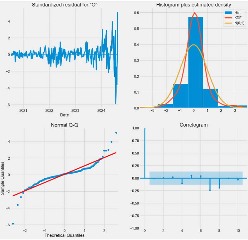
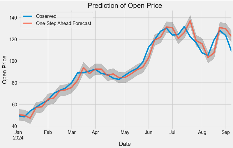
- One-step ahead ARIMA prediction of NVDA Open price in 2024
y_pred = result.get_prediction(start = pd.to_datetime('2024-01-01'), dynamic = False)

#visualize prediction of open price
pred_ci = y_pred.conf_int()
ax = x['2024':].plot(label = 'Observed')
y_pred.predicted_mean.plot(ax = ax, label = 'One-Step Ahead Forecast', alpha = .7, figsize = (10, 6))
ax.fill_between(pred_ci.index, pred_ci.iloc[:, 0], pred_ci.iloc[:, 1], color = 'k', alpha = .2)
plt.title("Prediction of Open Price")
ax.set_xlabel('Date')
ax.set_ylabel('Open Price')
plt.legend()
plt.show()
- Out-of-sample ARIMA prediction of NVDA Open price
#prediction of forecast
y_forecasted = y_pred.predicted_mean
y_truth = x['2024-03-01':]
mse = ((y_forecasted - y_truth) ** 2).mean()
print('The Mean Squared Error of our forecasts is {}'.format(round(mse, 2)))
print('The Root Mean Squared Error of our forecasts is {}'.format(round(np.sqrt(mse), 2)))

The Mean Squared Error of our forecasts is 37.26
The Root Mean Squared Error of our forecasts is 6.1

#visualize prediction of forecast
pred_uc = results.get_forecast(steps = 100)
pred_ci = pred_uc.conf_int()
ax = x.plot(label = 'Observed', figsize = (10,6))
pred_uc.predicted_mean.plot(ax = ax, label = 'Forecast')
ax.fill_between(pred_ci.index, pred_ci.iloc[:, 0], pred_ci.iloc[:, 1], color = 'k', alpha = .25)
plt.title("Forecast of Open Price")
ax.set_xlabel('Date')
ax.set_ylabel('Open Price')
plt.legend()
plt.show()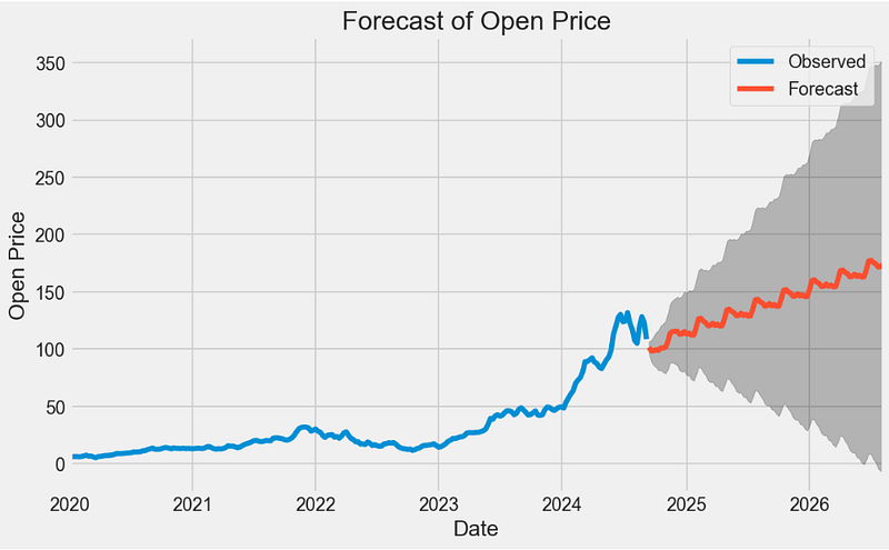
- Statistical testing of the above ARIMA forecast
# ADF Test
result = adfuller(x, autolag = 'AIC')
print(f'ADF Statistic: {result[0]}')
print(f'p-value: {result[1]}')
for key, value in result[4].items():
    print('Critial Values:')
    print(f'   {key}, {value}')

# KPSS Test
result = kpss(x, regression = 'c')
print('\nKPSS Statistic: %f' % result[0])
print('p-value: %f' % result[1])
for key, value in result[3].items():
    print('Critial Values:')
    print(f'   {key}, {value}')

# KPSS Test
result = kpss(x, regression = 'c')
print('\nKPSS Statistic: %f' % result[0])
print('p-value: %f' % result[1])
for key, value in result[3].items():
    print('Critial Values:')
    print(f'   {key}, {value}')

ADF Statistic: 0.00829081706485982
p-value: 0.959212383816871
Critial Values:
   1%, -3.4592326027153493
Critial Values:
   5%, -2.8742454699025872
Critial Values:
   10%, -2.5735414688888465

KPSS Statistic: 1.515224
p-value: 0.010000
Critial Values:
   10%, 0.347
Critial Values:
   5%, 0.463
Critial Values:
   2.5%, 0.574
Critial Values:
1%, 0.739- The p-value obtained by the ADF test should be less than the significance level 0.05 in order to reject the null hypothesis. It appears that the ARIMA prediction is not stationary since p=0.959.
- The KPSS test yields p=0.01. We can see from the p-value and critical values that we should reject the null of stationarity because the p-value is less than 5%.
Backtesting Logistic Regression with Technical Indicators [18]
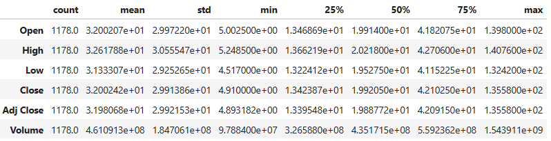
- Copying the input NVDA data
df=data.copy()

df.describe().T
- Calculating the RSI, MACD, SMA, and EMA indicators with default parameters
# Calculate RSI (Relative Strength Index)
def calculate_rsi(data, window=14):
    delta = data["Close"].diff(1)
    gain = delta.where(delta > 0, 0)
    loss = -delta.where(delta < 0, 0)

    avg_gain = gain.rolling(window=window, min_periods=1).mean()
    avg_loss = loss.rolling(window=window, min_periods=1).mean()

    rs = avg_gain / avg_loss
    rsi = 100 - (100 / (1 + rs))

    return rsi


df["RSI"] = calculate_rsi(df)


#Calculate MACD & Signal_Line

def calculate_macd(data, short_window=12, long_window=26):
    ema_short = data["Close"].ewm(span=short_window, min_periods=1, adjust=False).mean()
    ema_long = data["Close"].ewm(span=long_window, min_periods=1, adjust=False).mean()

    macd = ema_short - ema_long
    signal_line = macd.ewm(span=9, min_periods=1, adjust=False).mean()

    return macd, signal_line


df["MACD"], df["Signal_Line"] = calculate_macd(df)

#Calculate SMA

def calculate_sma(data, window=20):
    sma = data["Close"].rolling(window=window, min_periods=1).mean()
    return sma


df["SMA"] = calculate_sma(df)

#Calculate EMA

def calculate_ema(data, window=24):
    ema = data["Close"].ewm(span=window, min_periods=1,
              adjust=False).mean()
    return ema


df["EMA"] = calculate_ema(df)

#Calculate the Trading Signal

df["Signal"] = np.where(
    (df["RSI"] > 30) & (df["MACD"] > df["Signal_Line"])
    & (df["Close"] > df["SMA"]) & (df["Close"] > df["EMA"]),1,0)

df = df.dropna()- Splitting the data into training and testing sets, creating and training a Logistic Regression (LR) model, generating predictions on the test data, calculating ROC curve and AUC, backtesting the trading strategy, calculate cumulative returns, and plotting ML results
def build_model():
# Split the data into training and testing sets
train_size = int(0.8 * len(X))
X_train, X_test, y_train, y_test = (
X[:train_size],
X[train_size:],
y[:train_size],
y[train_size:],
)
# Create and train a Logistic Regression model
model = LogisticRegression()
model.fit(X_train, y_train)
# Generate predictions on the test data
y_pred = model.predict(X_test)
# Calculate accuracy
accuracy = accuracy_score(y_test, y_pred)
plt.figure(figsize=(4, 2))
coef_values = list(abs(model.coef_[0]))
feature_names = ["RSI", "MACD", "SMA", "EMA"]
plt.barh(feature_names, sorted(coef_values, reverse=False),
color="purple")
plt.xlabel("Coefficient Value")
plt.ylabel("Feature")
plt.title("Variable Importance (Coefficients)")
#plt.show()
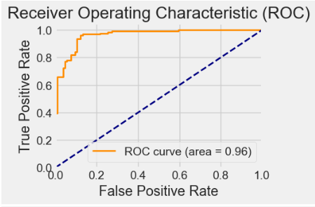
# Calculate ROC curve and AUC
y_prob = model.predict_proba(X_test)[:, 1]
fpr, tpr, _ = roc_curve(y_test, y_prob)
roc_auc = auc(fpr, tpr)
# Calculate and plot the confusion matrix
cm = confusion_matrix(y_test, y_pred)
plt.figure(figsize=(4, 3))
sns.heatmap(cm, annot=True, fmt="d", cmap="Blues", annot_kws={"size": 8})
plt.xlabel("Predicted")
plt.ylabel("Actual")
plt.title("Confusion Matrix")
plt.show()
# Backtesting the trading strategy
df["Strategy_Return"] = df["Close"].pct_change() * df["Signal"].shift(1)
df["Buy_Hold_Return"] = df["Close"].pct_change()
# Calculate cumulative returns
df["Cumulative_Strategy_Return"] = (1 + df["Strategy_Return"]).cumprod()
df["Cumulative_Buy_Hold_Return"] = (1 + df["Buy_Hold_Return"]).cumprod()
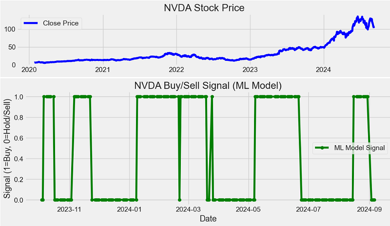
# Plot the stock's closing price, RSI, MACD, SMA, and EMA
plt.figure(figsize=(12, 6))
plt.subplot(3, 1, 1)
plt.plot(df["Close"], label="Close Price", color="blue")
plt.title(f"{stock_symbol} Stock Price")
plt.legend()
# Plot the buy/sell signals generated by the machine learning model
plt.figure(figsize=(12, 4))
plt.plot(
df.index[train_size:], y_pred, label="ML Model Signal", color="green", marker="o"
)
plt.title(f"{stock_symbol} Buy/Sell Signal (ML Model)")
plt.xlabel("Date")
plt.ylabel("Signal (1=Buy, 0=Hold/Sell)")
plt.legend()
# Plot ROC curve
plt.figure(figsize=(4, 3))
plt.plot(
fpr,
tpr,
color="darkorange",
lw=2,
label="ROC curve (area = {:.2f})".format(roc_auc),
)
plt.plot([0, 1], [0, 1], color="navy", lw=2, linestyle="--")
plt.xlim([0.0, 1.0])
plt.ylim([0.0, 1.05])
plt.xlabel("False Positive Rate")
plt.ylabel("True Positive Rate")
plt.title("Receiver Operating Characteristic (ROC)")
plt.legend(loc="lower right")
# Plot cumulative returns of the strategy and buy-and-hold
plt.figure(figsize=(12, 6))
plt.plot(
df.index, df["Cumulative_Strategy_Return"], label="Strategy Return", color="green"
)
plt.plot(
df.index,
df["Cumulative_Buy_Hold_Return"],
label="Buy and Hold Return",
color="blue",
)
plt.title("Cumulative Returns")
plt.xlabel("Date")
plt.ylabel("Cumulative Return")
plt.legend()
# Display accuracy
print(f"Model Accuracy: {accuracy * 100:.2f}%")
plt.show()
X = df[["RSI", "MACD", "SMA", "EMA"]].values
y = df["Signal"].values
# call the function
from sklearn.linear_model import LogisticRegression
from sklearn.metrics import accuracy_score
from sklearn.metrics import roc_curve
from sklearn.metrics import auc
from sklearn.metrics import confusion_matrix
stock_symbol='NVDA'
build_model()
Model Accuracy: 86.27%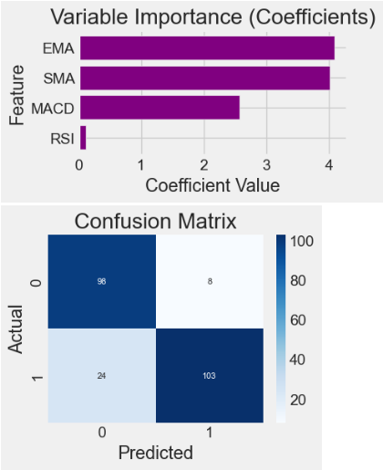
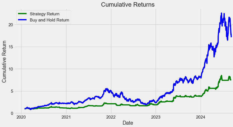
- It is clear that the proposed strategy underperforms about 10% of “buy-and-hold” in terms of expected returns.
Multiple Supervised ML Classification Algorithms with Technical Indicators [19]
- Importing the necessary Python libraries and reading the input NVDA stock data from 2022–01–01 to 2024–04–18
# Load packages

import numpy as np
import pandas as pd
from pandas import read_csv, set_option
from pandas.plotting import scatter_matrix
import matplotlib.pyplot as plt
import seaborn as sns
from sklearn.tree import DecisionTreeClassifier
from sklearn.neighbors import KNeighborsClassifier
from sklearn.linear_model import LogisticRegression
from sklearn.preprocessing import StandardScaler
from sklearn.naive_bayes import GaussianNB
from sklearn.svm import SVC
from sklearn.neural_network import MLPClassifier
from sklearn.pipeline import Pipeline
from sklearn.discriminant_analysis import LinearDiscriminantAnalysis
from sklearn.model_selection import GridSearchCV, train_test_split, KFold, cross_val_score
from sklearn.metrics import confusion_matrix, classification_report, accuracy_score
from sklearn.ensemble import GradientBoostingClassifier, AdaBoostClassifier, ExtraTreesClassifier, RandomForestClassifier

import pandas as pd
import numpy as np
symbols = ['NVDA']
start_date = '2022-01-01'
end_date = '2024-04-18'

dataset = yf.download(symbols, start=start_date, end=end_date)- Computing the following technical indicators with trading signals, excluding columns that are not needed for our prediction while dropping NaN values if any
# Create short simple moving average over a short 10-day-window
dataset['short_mvg'] = dataset['Close'].rolling(window=10, min_periods=1, center=False).mean()

# Create long simple moving average over a long 60-day-window
dataset['long_mvg'] = dataset['Close'].rolling(window=60, min_periods=1, center=False).mean()

# Create the signals
dataset['signal'] = np.where(dataset['short_mvg'] > dataset['long_mvg'], 1.0, 0.0)

#calculation of exponential moving average
def EMA(df, n):
    EMA = pd.Series(df['Close'].ewm(span=n, min_periods=n).mean(), name='EMA_' + str(n))
    return EMA
dataset['EMA10'] = EMA(dataset, 10)
dataset['EMA30'] = EMA(dataset, 30)
dataset['EMA200'] = EMA(dataset, 200)
dataset.head()

#calculation of rate of change
def ROC(df, n):
    M = df.diff(n - 1)
    N = df.shift(n - 1)
    ROC = pd.Series(((M / N) * 100), name = 'ROC_' + str(n))
    return ROC
dataset['ROC10'] = ROC(dataset['Close'], 10)
dataset['ROC30'] = ROC(dataset['Close'], 30)

#Calculation of price momentum
def MOM(df, n):
    MOM = pd.Series(df.diff(n), name='Momentum_' + str(n))
    return MOM
dataset['MOM10'] = MOM(dataset['Close'], 10)
dataset['MOM30'] = MOM(dataset['Close'], 30)

#calculation of relative strength index
def RSI(series, period):
 delta = series.diff().dropna()
 u = delta * 0
 d = u.copy()
 u[delta > 0] = delta[delta > 0]
 d[delta < 0] = -delta[delta < 0]
 u[u.index[period-1]] = np.mean( u[:period] ) #first value is sum of avg gains
 u = u.drop(u.index[:(period-1)])
 d[d.index[period-1]] = np.mean( d[:period] ) #first value is sum of avg losses
 d = d.drop(d.index[:(period-1)])
 rs = u.ewm(com=period-1, adjust=False).mean() / \
 d.ewm(com=period-1, adjust=False).mean()
 return 100 - 100 / (1 + rs)
dataset['RSI10'] = RSI(dataset['Close'], 10)
dataset['RSI30'] = RSI(dataset['Close'], 30)
dataset['RSI200'] = RSI(dataset['Close'], 200)

#calculation of stochastic osillator.

def STOK(close, low, high, n):
 STOK = ((close - low.rolling(n).min()) / (high.rolling(n).max() - low.rolling(n).min())) * 100
 return STOK

def STOD(close, low, high, n):
 STOK = ((close - low.rolling(n).min()) / (high.rolling(n).max() - low.rolling(n).min())) * 100
 STOD = STOK.rolling(3).mean()
 return STOD

dataset['%K10'] = STOK(dataset['Close'], dataset['Low'], dataset['High'], 10)
dataset['%D10'] = STOD(dataset['Close'], dataset['Low'], dataset['High'], 10)
dataset['%K30'] = STOK(dataset['Close'], dataset['Low'], dataset['High'], 30)
dataset['%D30'] = STOD(dataset['Close'], dataset['Low'], dataset['High'], 30)
dataset['%K200'] = STOK(dataset['Close'], dataset['Low'], dataset['High'], 200)
dataset['%D200'] = STOD(dataset['Close'], dataset['Low'], dataset['High'], 200)

#Calculation of moving average
def MA(df, n):
    MA = pd.Series(df['Close'].rolling(n, min_periods=n).mean(), name='MA_' + str(n))
    return MA
dataset['MA21'] = MA(dataset, 10)
dataset['MA63'] = MA(dataset, 30)
dataset['MA252'] = MA(dataset, 200)

#excluding columns that are not needed for our prediction.
dataset=dataset.drop(['High','Low','Open','short_mvg','long_mvg'], axis=1)

dataset = dataset.dropna(axis=0)- Plotting the correlation heatmap
# correlation
correlation = dataset.corr()
plt.figure(figsize=(20,20))
plt.title('Correlation Matrix')
sns.heatmap(correlation, vmax=1, square=True,annot=True,cmap='cubehelix')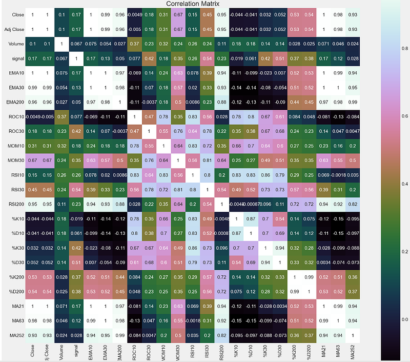
- Splitting the input dataset into training/validation sets with validation_size = 0.2
# split out validation dataset for the end
subset_dataset= dataset.iloc[-100000:]
Y= subset_dataset["signal"]
X = subset_dataset.loc[:, dataset.columns != 'signal']
validation_size = 0.2
seed = 1
X_train, X_validation, Y_train, Y_validation = train_test_split(X, Y, test_size=validation_size, random_state=1)- Training and comparing multiple supervised ML classification algorithms
# test options for classification
num_folds = 10
seed = 7
scoring = 'accuracy'

# spot check the algorithms
models = []
models.append(('LR', LogisticRegression(n_jobs=-1)))
models.append(('LDA', LinearDiscriminantAnalysis()))
models.append(('KNN', KNeighborsClassifier()))
models.append(('CART', DecisionTreeClassifier()))
models.append(('NB', GaussianNB()))
# Neural Network
models.append(('NN', MLPClassifier()))
# Ensable Models
# Boosting methods
models.append(('AB', AdaBoostClassifier()))
models.append(('GBM', GradientBoostingClassifier()))
# Bagging methods
models.append(('RF', RandomForestClassifier(n_jobs=-1)))

results = []
names = []
for name, model in models:
    kfold = KFold(n_splits=num_folds)
    cv_results = cross_val_score(model, X_train, Y_train, cv=kfold, scoring=scoring)
    results.append(cv_results)
    names.append(name)
    msg = "%s: %f (%f)" % (name, cv_results.mean(), cv_results.std())
    print(msg)

LR: 0.889655 (0.069958)
LDA: 0.969885 (0.027705)
KNN: 0.822299 (0.084645)
CART: 0.933103 (0.036521)
NB: 0.852529 (0.074317)
NN: 0.759195 (0.250235)
AB: 0.973333 (0.035901)
GBM: 0.973333 (0.029059)
RF: 0.956667 (0.047258)

# compare algorithms
fig = plt.figure()
fig.suptitle('Algorithm Comparison')
ax = fig.add_subplot(111)
plt.boxplot(results)
ax.set_xticklabels(names)
fig.set_size_inches(15,8)
plt.show()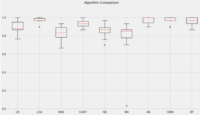
- Selecting the Random Forest (RF) classifier to perform Grid Search HPO
# Grid Search: Random Forest Classifier
'''
n_estimators : int (default=100)
    The number of boosting stages to perform.
    Gradient boosting is fairly robust to over-fitting so a large number usually results in better performance.
max_depth : integer, optional (default=3)
    maximum depth of the individual regression estimators.
    The maximum depth limits the number of nodes in the tree.
    Tune this parameter for best performance; the best value depends on the interaction of the input variables
criterion : string, optional (default=”gini”)
    The function to measure the quality of a split.
    Supported criteria are “gini” for the Gini impurity and “entropy” for the information gain.

'''
scaler = StandardScaler().fit(X_train)
rescaledX = scaler.transform(X_train)
n_estimators = [20,80]
max_depth= [5,10]
criterion = ["gini","entropy"]
param_grid = dict(n_estimators=n_estimators, max_depth=max_depth, criterion = criterion )
model = RandomForestClassifier(n_jobs=-1)
kfold = KFold(n_splits=num_folds)
grid = GridSearchCV(estimator=model, param_grid=param_grid, scoring=scoring, cv=kfold)
grid_result = grid.fit(rescaledX, Y_train)

#Print Results
print("Best: %f using %s" % (grid_result.best_score_, grid_result.best_params_))
means = grid_result.cv_results_['mean_test_score']
stds = grid_result.cv_results_['std_test_score']
params = grid_result.cv_results_['params']
ranks = grid_result.cv_results_['rank_test_score']
for mean, stdev, param, rank in zip(means, stds, params, ranks):
    print("#%d %f (%f) with: %r" % (rank, mean, stdev, param))

Best: 0.970000 using {'criterion': 'entropy', 'max_depth': 10, 'n_estimators': 20}
#6 0.953333 (0.054160) with: {'criterion': 'gini', 'max_depth': 5, 'n_estimators': 20}
#6 0.953333 (0.054160) with: {'criterion': 'gini', 'max_depth': 5, 'n_estimators': 80}
#5 0.956667 (0.053852) with: {'criterion': 'gini', 'max_depth': 10, 'n_estimators': 20}
#4 0.960000 (0.044222) with: {'criterion': 'gini', 'max_depth': 10, 'n_estimators': 80}
#8 0.950000 (0.050000) with: {'criterion': 'entropy', 'max_depth': 5, 'n_estimators': 20}
#2 0.963333 (0.043333) with: {'criterion': 'entropy', 'max_depth': 5, 'n_estimators': 80}
#1 0.970000 (0.031447) with: {'criterion': 'entropy', 'max_depth': 10, 'n_estimators': 20}
#2 0.963333 (0.043333) with: {'criterion': 'entropy', 'max_depth': 10, 'n_estimators': 80}

# prepare model
model = RandomForestClassifier(criterion='entropy', n_estimators=20,max_depth=10,n_jobs=-1) # rbf is default kernel
#model = GaussianNB()
model.fit(X_train, Y_train)

RandomForestClassifier:
RandomForestClassifier(criterion='entropy', max_depth=10, n_estimators=20,
                       n_jobs=-1)

# estimate accuracy on validation set
predictions = model.predict(X_validation)
print(accuracy_score(Y_validation, predictions))
print(confusion_matrix(Y_validation, predictions))
print(classification_report(Y_validation, predictions))

0.9466666666666667
[[ 6  2]
 [ 2 65]]
              precision    recall  f1-score   support

         0.0       0.75      0.75      0.75         8
         1.0       0.97      0.97      0.97        67

    accuracy                           0.95        75
   macro avg       0.86      0.86      0.86        75
weighted avg 0.95 0.95 0.95 75- Plotting the HPO RF confusion matrix, variable importance and strategy returns vs actual returns after backtesting
df_cm = pd.DataFrame(confusion_matrix(Y_validation, predictions), columns=np.unique(Y_validation), index = np.unique(Y_validation))
df_cm.index.name = 'Actual'
df_cm.columns.name = 'Predicted'
sns.heatmap(df_cm, cmap="Blues", annot=True,annot_kws={"size": 16})# font sizes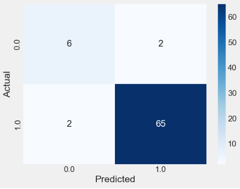
Importance = pd.DataFrame({'Importance':model.feature_importances_*100}, index=X.columns)
Importance.sort_values('Importance', axis=0, ascending=True).plot(kind='barh', color='r' )
plt.xlabel('Variable Importance')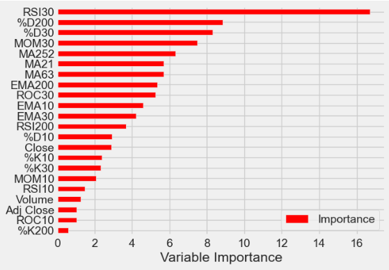
#Create column for Strategy Returns by multiplying the daily returns by the position that was held at close
#of business the previous day
backtestdata = pd.DataFrame(index=X_validation.index)
#backtestdata = pd.DataFrame()
backtestdata['signal_pred'] = predictions
backtestdata['signal_actual'] = Y_validation
backtestdata['Market Returns'] = X_validation['Close'].pct_change()
backtestdata['Actual Returns'] = backtestdata['Market Returns'] * backtestdata['signal_actual'].shift(1)
backtestdata['Strategy Returns'] = backtestdata['Market Returns'] * backtestdata['signal_pred'].shift(1)
backtestdata=backtestdata.reset_index()
backtestdata.head()
backtestdata[['Strategy Returns','Actual Returns']].cumsum().hist()
backtestdata[['Strategy Returns','Actual Returns']].cumsum().plot()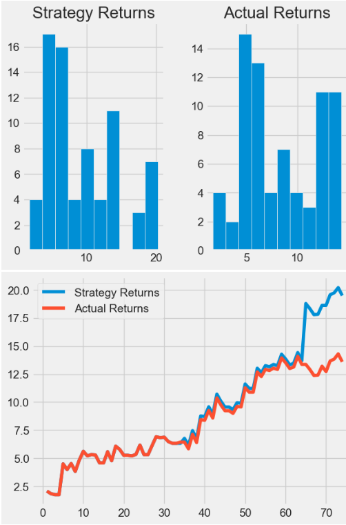
- It is clear that the proposed NVDA trading strategy outperforms 5% actual returns after backtesting.
BTC-USD Price Prediction using LSTM
- Let’s discuss an approach for predicting the price of BTC-USD using LSTM [20–24].
- Challenge: Today’s cryptocurrency has a high market value, and the price of BTC-USD fluctuates dramatically. Because of its fluctuations, an automated tool for predicting bitcoin on the stock market is required.
- Motivation: Deep learning LSTM neural networks solve the problem of vanishing gradients in RNNs by replacing nodes in the RNN with memory cells and a gating mechanism. They have recently gained popularity in deep learning because of their ability to overcome the limitations of existing NN architecture when learning over long sequences. In fact, LSTMs are explicitly designed to avoid the problem of long-term dependency [26].
- Importing the necessary Python libraries and reading the input BTC-USD data from 2023–01–1 to 2024–09–09
import numpy as np
import pandas as pd
import matplotlib.pyplot as plt
from keras.models import Sequential
from keras.layers import Dense, LSTM
import math
from sklearn.preprocessing import MinMaxScaler,StandardScaler,RobustScaler
import datetime
import pandas as pd
pd.set_option('display.max_columns', None)
pd.set_option('display.max_rows', None)
#Reading and Displaying BTC Time Series Data

import yfinance as yf

start_date = "2023-01-1"

btc = yf.download('BTC-USD',
                      start=start_date,
                      progress=False)

btc.tail()

           Open         High         Low          Close        Adj Close    Volume
Date
2024-09-04 57430.347656 58511.570312 55673.164062 57971.539062 57971.539062 35627680312
2024-09-05 57971.703125 58300.582031 55712.453125 56160.488281 56160.488281 31030280656
2024-09-06 56160.191406 56976.109375 52598.699219 53948.753906 53948.753906 49361693566
2024-09-07 53949.085938 54838.144531 53740.070312 54139.687500 54139.687500 19061486526
2024-09-08 54148.867188 54541.875000 54009.578125 54381.371094 54381.371094 16332175360
2024-09-09 54864.863281 55315.097656 54611.968750 55164.128906 55164.128906 22548137984

#  Plotting date vs the close market stock price
final_data=btc
final_data['Date'] = btc.index

final_data.plot('Date','Close',color="red",figsize=(12,6))
plt.title('BTC-USD Close Price')
plt.grid(color='grey')

new_data = final_data.tail(60)
new_data.plot('Date','Close',color="green",figsize=(12,6),lw=3)
plt.grid(color='grey')
plt.show()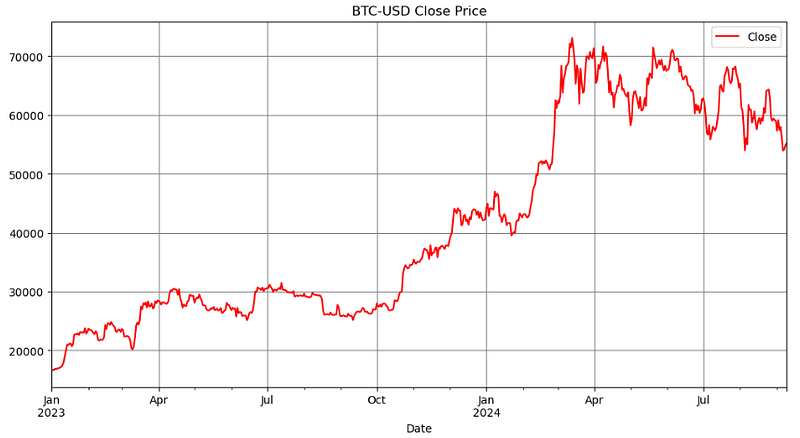
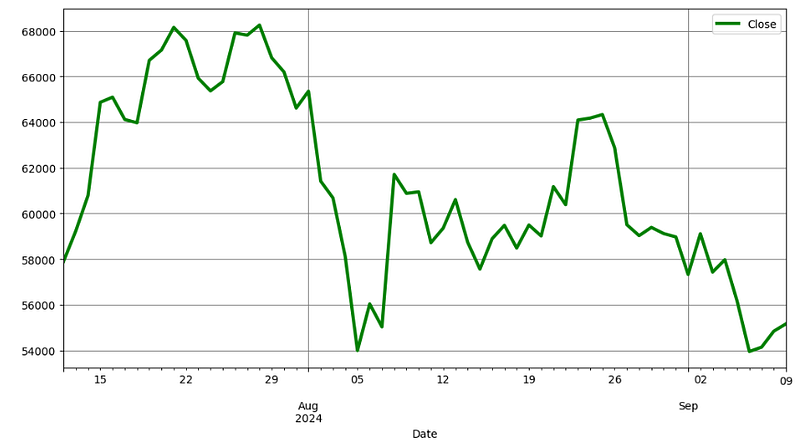
- Preparing the training data for LSTM [20]
#Creating a new Dataframe and Training data
# 1. Filter out the closing market price data
close_data = final_data.filter(['Close'])

# 2. Convert the data into array for easy evaluation
dataset = close_data.values
datasetindex=close_data.index

# 3. Scale/Normalize the data to make all values between 0 and 1
scaler = RobustScaler()
scaled_data = scaler.fit_transform(dataset)

# 4. Creating training data size : 80% of the data
training_data_len = math.ceil(len(dataset) *.8)
train_data = scaled_data[0:training_data_len  , : ]

# 5. Separating the data into x and y data
x_train_data=[]
y_train_data =[]
for i in range(30,len(train_data)):
    x_train_data=list(x_train_data)
    y_train_data=list(y_train_data)
    x_train_data.append(train_data[i-30:i,0])
    y_train_data.append(train_data[i,0])

    # 6. Converting the training x and y values to numpy arrays
    x_train_data1, y_train_data1 = np.array(x_train_data), np.array(y_train_data)

    # 7. Reshaping training s and y data to make the calculations easier
x_train_data2 = np.reshape(x_train_data1, (x_train_data1.shape[0],x_train_data1.shape[1],1))- Building the LSTM Sequential model
#Building LSTM Model
model = Sequential()
model.add(LSTM(units=50, return_sequences=True,input_shape=(x_train_data2.shape[1],1)))
model.add(LSTM(units=50, return_sequences=False))
model.add(Dense(units=25))
model.add(Dense(units=1))

model.summary()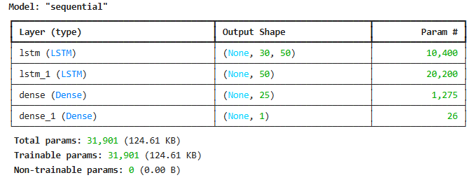
- Compiling and fitting the LSTM model by optimizing the input parameters batch_size and epochs to address a bias-variance trade-off
model.compile(optimizer='adam', loss='mean_squared_error')
history=model.fit(x_train_data2, y_train_data1, batch_size=1, epochs=50)

poch 1/50
464/464 ━━━━━━━━━━━━━━━━━━━━ 6s 6ms/step - loss: 0.0183
Epoch 2/50
464/464 ━━━━━━━━━━━━━━━━━━━━ 3s 6ms/step - loss: 0.0048
Epoch 3/50
464/464 ━━━━━━━━━━━━━━━━━━━━ 3s 6ms/step - loss: 0.0043
Epoch 4/50
464/464 ━━━━━━━━━━━━━━━━━━━━ 3s 7ms/step - loss: 0.0035
Epoch 5/50
464/464 ━━━━━━━━━━━━━━━━━━━━ 3s 6ms/step - loss: 0.0026

........................................

Epoch 43/50
464/464 ━━━━━━━━━━━━━━━━━━━━ 3s 7ms/step - loss: 0.0014
Epoch 44/50
464/464 ━━━━━━━━━━━━━━━━━━━━ 4s 8ms/step - loss: 0.0014
Epoch 45/50
464/464 ━━━━━━━━━━━━━━━━━━━━ 4s 8ms/step - loss: 0.0016
Epoch 46/50
464/464 ━━━━━━━━━━━━━━━━━━━━ 3s 6ms/step - loss: 0.0014
Epoch 47/50
464/464 ━━━━━━━━━━━━━━━━━━━━ 3s 7ms/step - loss: 0.0016
Epoch 48/50
464/464 ━━━━━━━━━━━━━━━━━━━━ 4s 8ms/step - loss: 0.0011
Epoch 49/50
464/464 ━━━━━━━━━━━━━━━━━━━━ 4s 8ms/step - loss: 0.0016
Epoch 50/50
464/464 ━━━━━━━━━━━━━━━━━━━━ 3s 7ms/step - loss: 0.0015- Plotting the LSTM MSE Loss vs Epoch curve
plt.figure(figsize=(10,6))
plt.plot(history.history['loss'], label='train')
plt.legend()
plt.xlabel('Epoch')
plt.ylabel('MSE Loss')
plt.title('LSTM BTC-USD Prediction')
plt.grid(color='grey')
plt.show()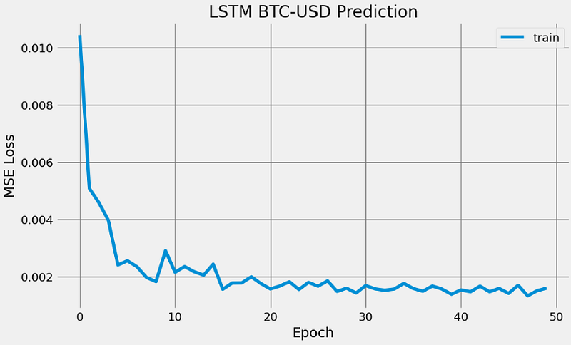
- Making LSTM predictions on the testing data to perform validation QC
#Testing the model on testing data
# 1. Creating a dataset for testing
test_data = scaled_data[training_data_len - 30: , : ]
test_index=datasetindex[training_data_len - 30:]
x_test = []
y_test =  dataset[training_data_len : , : ]
for i in range(30,len(test_data)):
    x_test.append(test_data[i-30:i,0])

# 2.  Convert the values into arrays for easier computation
x_test = np.array(x_test)
x_test = np.reshape(x_test, (x_test.shape[0],x_test.shape[1],1))

# 3. Making predictions on the testing data
predictions = model.predict(x_test)
predictions = scaler.inverse_transform(predictions)

#Error Calculation
rmse=np.sqrt(np.mean(((predictions- y_test)**2)))
print(rmse)

2021.637269498445

plt.figure(figsize=(10,6))
plt.plot(predictions,label='predictions')
plt.plot(y_test,label='test data')
plt.legend(loc="upper left")
plt.title("BTC-USD Test Data vs LSTM Predictions")
plt.xlabel("Forecast Day")
plt.ylabel("Price USD")
plt.grid(color='grey')
plt.show()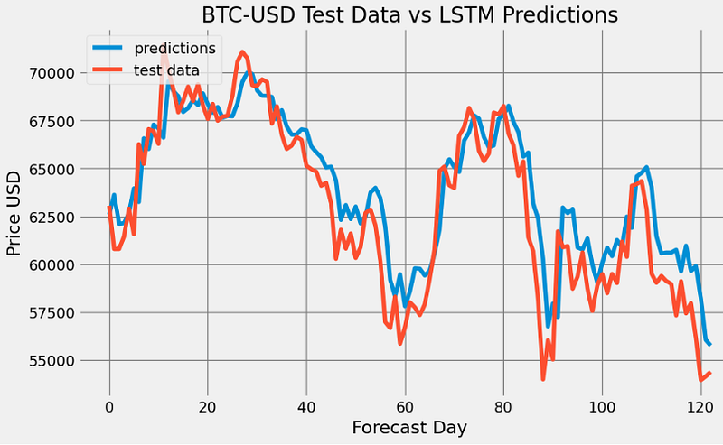
- These tests show that the trained LSTM model performs well in BTC-USD Close price prediction.
AAPL Price Prediction using LSTM
- Finally, let’s build a Keras LSTM model [20–23] to forecast AAPL stock prices [24].
- Challenge: Overfitting is a general problem for NNs, where they overfit to only the training data and get low generalization performance. LSTM often suffers from overfitting because of its complex and expressive structure.
- Reading and plotting the input stock data
df = yf.download('AAPL', start='2020-01-01')

plt.figure(figsize=(10,6))
plt.title('AAPL Close Price History')
plt.plot(df['Close'],linewidth=3)
plt.xlabel('Date', fontsize=18)
plt.ylabel('Close Price USD ($)', fontsize=18)
plt.grid(lw=3)
plt.show()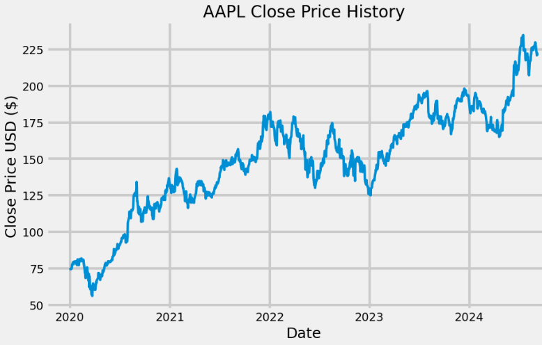
- Creating the training data for LSTM
# Create a new dataframe with only the 'Close column
data = df.filter(['Close'])
# Convert the dataframe to a numpy array
dataset = data.values
# Get the number of rows to train the model on
training_data_len = int(np.ceil( len(dataset) * .7 ))

training_data_len
825

# Scale the data
from sklearn.preprocessing import StandardScaler

#scaler = MinMaxScaler(feature_range=(0,1))
scaler = StandardScaler()
scaled_data = scaler.fit_transform(dataset)

# Create the scaled training data set
train_data = scaled_data[0:int(training_data_len), :]
# Split the data into x_train and y_train data sets
x_train = []
y_train = []

for i in range(60, len(train_data)):
    x_train.append(train_data[i-60:i, 0])
    y_train.append(train_data[i, 0])
    if i<= 61:
        print(x_train)
        print(y_train)
        print()

# Convert the x_train and y_train to numpy arrays
x_train, y_train = np.array(x_train), np.array(y_train)

# Reshape the data
x_train = np.reshape(x_train, (x_train.shape[0], x_train.shape[1], 1))- Building the LSTM model with optimal parameters batch_size=4 and epochs=5 to circumvent data overfitting
from keras.models import Sequential
from keras.layers import Dense, LSTM

# Build the LSTM model
model = Sequential()
model.add(LSTM(128, return_sequences=True, input_shape= (x_train.shape[1], 1)))
model.add(LSTM(64, return_sequences=False))
model.add(Dense(25))
model.add(Dense(1))

# Compile the model
model.compile(optimizer='adam', loss='mean_squared_error')

# Train the model
history=model.fit(x_train, y_train, batch_size=4, epochs=5)

Epoch 1/5
192/192 ━━━━━━━━━━━━━━━━━━━━ 6s 16ms/step - loss: 0.0503
Epoch 2/5
192/192 ━━━━━━━━━━━━━━━━━━━━ 3s 16ms/step - loss: 0.0166
Epoch 3/5
192/192 ━━━━━━━━━━━━━━━━━━━━ 3s 16ms/step - loss: 0.0136
Epoch 4/5
192/192 ━━━━━━━━━━━━━━━━━━━━ 3s 16ms/step - loss: 0.0089
Epoch 5/5
192/192 ━━━━━━━━━━━━━━━━━━━━ 3s 16ms/step - loss: 0.0080- Plotting the LSTM MSE Loss vs Epoch curve
plt.figure(figsize=(10,6))
plt.plot(history.history['loss'], label='train')
plt.legend()
plt.xlabel('Epoch')
plt.ylabel('MSE Loss')
plt.title('LSTM AAPL Prediction')
plt.show()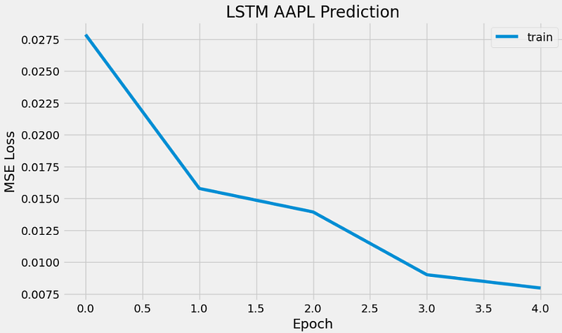
- Using test data to validate LSTM predictions
# Create the testing data set

test_data = scaled_data[training_data_len - 60: , :]
# Create the data sets x_test and y_test
x_test = []
y_test = dataset[training_data_len:, :]
for i in range(60, len(test_data)):
    x_test.append(test_data[i-60:i, 0])

# Convert the data to a numpy array
x_test = np.array(x_test)

# Reshape the data
x_test = np.reshape(x_test, (x_test.shape[0], x_test.shape[1], 1 ))

# Get the models predicted price values
predictions = model.predict(x_test)
predictions = scaler.inverse_transform(predictions)

# Get the root mean squared error (RMSE)
rmse = np.sqrt(np.mean(((predictions - y_test) ** 2)))
rmse

4.2125933122206

# Plot the data
train = data[:training_data_len]
valid = data[training_data_len:]
valid['Predictions'] = predictions
# Visualize the data
plt.figure(figsize=(16,6))
plt.title('AAPL Close Price')
plt.xlabel('Date', fontsize=18)
plt.ylabel('Close Price USD ($)', fontsize=18)
plt.plot(train['Close'],linewidth=3)
plt.plot(valid[['Close', 'Predictions']],linewidth=3)
plt.legend(['Train', 'Val', 'Predictions'], loc='lower right')
plt.grid(lw=3)
plt.show()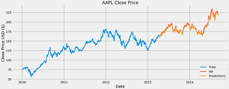
plt.xlabel('Forecast Day', fontsize=18)
plt.ylabel('Close Price USD ($)', fontsize=18)
plt.plot(predictions)
plt.plot(y_test)
plt.title('AAPL Test Data LSTM Prediction')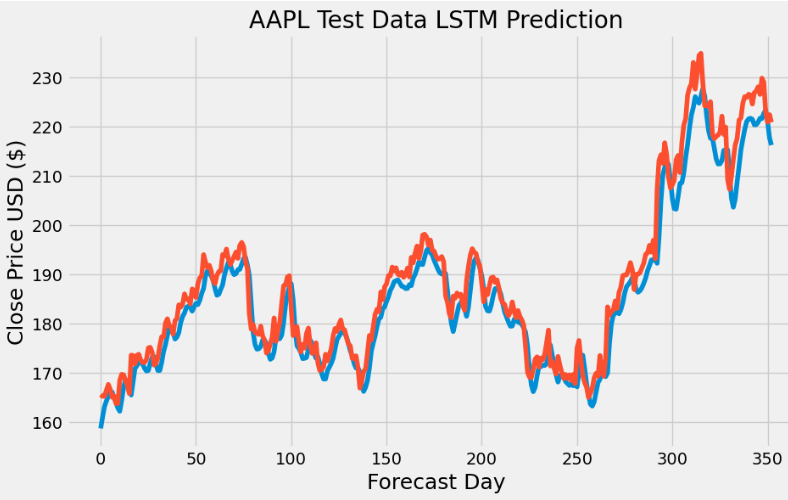
- In this study, we have addressed the LSTM data overfitting issues by slightly increasing batch_size>1 (thereby reducing the high-frequency content) while reducing the number of epochs (early stop).
Conclusions
TSLA Linear/Nonlinear Trend Detection with Time Dummy
- Provided the time series doesn’t have any missing dates, we can create a time dummy by counting out the length of the series.
- The Linear Regression (LR) model assumes a linear relationship between the time variable and Close price. In the current study, this assumption is violated, leading to biased predictions of TSLA stock prices.
- Polynomial Regression (PR) provides more accurate predictions of TSLA prices than LR.
- The degree of the polynomial equation determines the level of nonlinearity in the price-time relationship.
- However, PR models have poor interpolatory and extrapolatory properties. Even a single outlier in the data can seriously mess up the results. Generally, high degree polynomials (n>>2) are notorious for oscillations between exact-fit values.
TSLA Linear Regression with Lagged Variables
- We have evaluated the LR model that captures the dynamic causal link between an observed stock price and several lagged observations (previous time steps). The core idea is that the current value of a time series can be expressed as a linear combination of its past values, with some random noise.
- Direct comparisons of the actual time series (i.e. test values against the test predictions), train/test data residuals for the LR model, and X-plots predictions vs test data predicted values do not deviate significantly from the actual test values.
- The following performance metrics give us a quantitative measure of how well the LR model predicts the time series data based on its lagged features
MAE: 5.59
MAPE: 0.03
MSE: 56.30
R^2 Score: 0.92- This result suggests that the LR model fits the Close price quite well and is a good predictor for the TSLA dataset.
BTC-USD Price Prediction & Algo-Trading Strategies using FB Prophet
- Prophet with the Box-Cox transformation and a cap or upper limit for the forecast yields the 1Y prediction with relatively narrow CI and can capture non-linearity in the trend of the data
- Adding the monthly/quarterly seasonality and US events reveals a fairly strong yearly seasonality and a somewhat increased frequency content with reasonable CI of the out-of-sample predictions.
- 1Y forecast (2022–2027 time interval): combining the Box-Cox transformation and HPO reduces MAE about 20 times.
- 2020–2027 Time Interval: Splitting the date index improves the in-sample goodness-of-fit of the Prophet forecast.
- The HPO-updated Prophet model and 1Y predictions yield
Mean Absolute Error: 13879.24
Mean Squared Error: 279497823.66
Root Mean Squared Error: 16718.19- Backtesting of algo-trading strategies result in the following expected returns
Hold = 6,049
Prophet = 62,849
Prophet Thresh = 23,986
Seasonality = 8,195
Optimized Prophet Thresh = 97,000- Prophet provides an interpretable decomposition of the data that is observed or forecasted into trend and multi-seasonal components.
- Different useful plotting options are available in Prophet: forecasts in terms of yhat/yhat_lower/yhat_upper, cross-validation metrics, Plotly plots with changepoints, etc.
NVDA Price Prediction using Auto-ARIMA, Supervised ML & Technical Indicators
- We have created the NVDA candlestick chart with top 5 simple moving averages (SMA 5, 20, 50, 200, 500) in Plotly.
- Auto-ARIMA Modeling results consist of the additive trend-seasonality decomposition using statsmodels, the autocorrelation function, an optimal parameter combination for Seasonal ARIMA without enforcing stationarity of time series, ARIMA Validation QC (standardized residuals, histogram plus estimated density, Normal Q-Q plot, and correlogram), one-step ahead ARIMA prediction in 2024 and out-of-sample 2Y ARIMA forecast of NVDA Open price.
The Mean Squared Error of our forecasts is 37.26
The Root Mean Squared Error of our forecasts is 6.1
# The trained ARIMA model
result = model.fit()
print(results.summary().tables[1])
==============================================================================
coef std err z P>|z| [0.025 0.975]
------------------------------------------------------------------------------
ar.L1 0.1853 0.063 2.932 0.003 0.061 0.309
ma.L1 0.3696 0.072 5.111 0.000 0.228 0.511
ar.S.L12 -0.1825 0.117 -1.565 0.118 -0.411 0.046
ma.S.L12 -0.6436 0.101 -6.399 0.000 -0.841 -0.446
sigma2 6.6759 0.276 24.223 0.000 6.136 7.216
==============================================================================- The p-value obtained by the ADF test should be less than the significance level 0.05 in order to reject the null hypothesis. It appears that the ARIMA prediction is not stationary since p=0.959.
- The KPSS test yields p=0.01. We can see from the p-value and critical values that we should reject the null of stationarity because the p-value is less than 5%.
- Backtesting Logistic Regression (LR) with Technical Indicators (RSI, MACD, SMA, and EMA): EMA is the most dominant feature, Model Accuracy is 86.27%, ROC area is 0.96. However, the LR-based algo-trading strategy underperforms about 10% of “buy-and-hold” in terms of expected returns.
- Multiple Supervised ML Classification Algorithms with 20 Popular Technical Indicators: RSI30 is the most dominant feature, Random Forest (RF) is the best performing binary classifier.
# ML mean accuracy score with std
msg = "%s: %f (%f)" % (name, cv_results.mean(), cv_results.std())
    print(msg)

LR: 0.889655 (0.069958)
LDA: 0.969885 (0.027705)
KNN: 0.822299 (0.084645)
CART: 0.933103 (0.036521)
NB: 0.852529 (0.074317)
NN: 0.759195 (0.250235)
AB: 0.973333 (0.035901)
GBM: 0.973333 (0.029059)
RF: 0.956667 (0.047258)- Results of RF Grid Search HPO:
# estimate accuracy on validation set
predictions = model.predict(X_validation)
print(accuracy_score(Y_validation, predictions))
print(confusion_matrix(Y_validation, predictions))
print(classification_report(Y_validation, predictions))

0.9466666666666667
[[ 6  2]
 [ 2 65]]
              precision    recall  f1-score   support

         0.0       0.75      0.75      0.75         8
         1.0       0.97      0.97      0.97        67

    accuracy                           0.95        75
   macro avg       0.86      0.86      0.86        75
weighted avg 0.95 0.95 0.95 75- The proposed RF-based NVDA algo-trading strategy outperforms 5% actual returns after backtesting.
BTC-USD & AAPL Price Prediction using LSTM
#BTC-USD Error Calculation
rmse=np.sqrt(np.mean(((predictions- y_test)**2)))
print(rmse)

2021.637269498445

# AAPL root mean squared error (RMSE)
rmse = np.sqrt(np.mean(((predictions - y_test) ** 2)))
rmse

4.2125933122206- In this study, we have addressed the LSTM data overfitting issues by slightly increasing batch_size>1 (thereby reducing the high-frequency content) while reducing the number of epochs (early stop).
- Our tests have shown that the trained LSTM models perform well in both BTC-USD and AAPL price prediction examples.
References
- Linear Regression With Time Series
- The Drawbacks of Linear Regression Models: Limitations and Their Impact on Accuracy
- Polynomial Regression Economies_of_Scale
- Polynomial Regression in Python
- Analyzing the Impact of Lagged Features in Time Series Forecasting: A Linear Regression Approach
- Simple Data Exploration and Lag Feature Regression
- Autoregressive (AR) Model for Time Series Forecasting
- FbProphet and Plotly Example
- Tutorial: Time Series Forecasting with Prophet
- Bitcoin Price Forecasting using FB PROPHET
- Getting Started Predicting Time Series Data with Facebook Prophet
- Microsoft Stock Price Prediction.ipynb
- Stock Price Forecast with Prophet.ipynb
- Is Facebook Prophet suited for doing good predictions in a real-world project?
- Stocks, Candlestick with volume in plotly
- Time-Series Analysis and Forecasting with Meta’s Prophet Library
- Stock Forecast with ProphetML
- MasterCard Stock Analysis
- Ethereum Price Prediction
- Stock Price Prediction using Python
- Stock Price Prediction using LSTM and its Implementation
- Bitcoin Price Prediction using LSTM
- Stock Market Analysis + Prediction using LSTM
- LSTM Model For Apple Stock Prediction
- Hands-On-Machine-Learning-for-Algorithmic-Trading
- Bitcoin Price Trend Prediction Using Deep Neural Network: Webology (ISSN: 1735–188X) Volume 19, Number 3, 2022.
Explore More
- DigHiSci Posts
- Full-Fledged Technical Analysis of Top Growth Stocks: Backtesting Volatility Resilience vs Profitability
- NVDA vs BTC Algorithmic Trading: Backtest BB, MACD & AO Trading Strategies
- Building Supervised Machine Learning Streamlit Web App
- NVIDIA Short-Term Stock Price Forecasting: SHAP Explainer, Lags, Optimized ML Regressors, Auto-ARIMA, Multi-Seasonal FB Prophet Tuning & LSTM
- An Integrated Quant Trading Analysis of US Big Techs using Quantstats, TA, PyPortfolioOpt, and FinanceToolkit
- BTC-USD Price Prediction using FB Prophet with Hyperparameter Optimization, Cross-Validation QC & Modified Algo-Trading Strategies
- NVDA Technical Analysis using 75 Simplified FinTA Indicators
- Vectorized Backtesting & Parameter Tuning of AutoARIMA SMA Strategy: BTC-Tech vs S&P 500
- Combining ARIMA, LSTM and Fourier Models with Technical Indicators for JPM Price Prediction and Backtesting
- BTC Price Prediction using FB Prophet
- Backtesting the NVIDIA Scalping Strategy with SPY Benchmark & VaR Simulations
- A Deeper Look at NVIDIA KST Algo-Trading Signals & Backtesting
- Algo-Trading NVIDIA with ADX & RSI Indicators
- An Algo-Trading Sneak Peek at Top AI-Powered Growth Stocks — 1. NVIDIA
Contacts
Disclaimer
- The following disclaimer clarifies that the information provided in this article is for educational use only and should not be considered financial or investment advice.
- The information provided does not take into account your individual financial situation, objectives, or risk tolerance.
- Any investment decisions or actions you undertake are solely your responsibility.
- You should independently evaluate the suitability of any investment based on your financial objectives, risk tolerance, and investment timeframe.
- It is recommended to seek advice from a certified financial professional who can provide personalized guidance tailored to your specific needs.
- The tools, data, content, and information offered are impersonal and not customized to meet the investment needs of any individual. As such, the tools, data, content, and information are provided solely for informational and educational purposes only.


