Vectorized Backtesting & Parameter Tuning of AutoARIMA SMA Strategy: BTC-Tech vs S&P 500

This post is about the vectorized backtesting of simple moving averages (SMA) based strategies with different lengths.
The objective is to find an optimal set of parameters by maximizing portfolio returns while outperforming the S&P 500.
Following the ML vectorized backtesting idea, our project aims to devise stock trading strategies beyond ad hoc price forecasts.
Specifically, the AutoARIMA model will be adopted to predict SMA trading decisions directly. We’ll provide ML SMA predictions for the optimum set of parameters by fitting the ML model to the training set.
In the sequel, we’ll use the EODHD SMA algorithm to backtest the expected returns of BTC-USD combined with top 3 tech stocks (NVDA, AMD, and MSFT).
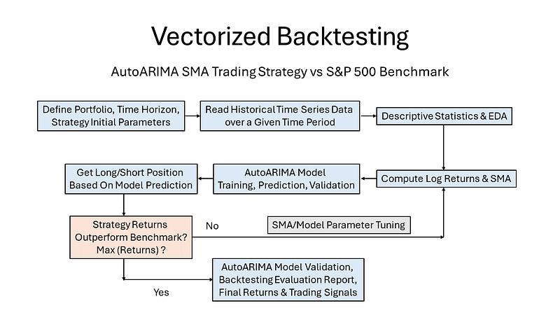
The entire workflow consists of the following steps (cf. the flowchart below):

Define our portfolio, time horizon, and strategy initial parameters
Read historical time series data using yfinance over a specific time period
Run the Pandas Exploratory Data Analysis (EDA) and examine the descriptive summary statistics.
Compute Log Returns and SMA.
Perform pmdarima AutoARIMA model training, prediction, and validation.
Comparing Returns per Stock using ARIMA forecast.
Comparing SPY vs ARIMA Overall Portfolio Returns (OPR).
If OPR(SPY) > OPR(ARIMA), then go to step 4 and update both the SMA length and AutoARIMA parameters (i.e. days_to_train and days_to_predict).
Output the full backtesting evaluation report with relevant plots.

Vectorized Backtesting AutoARIMA SMA Trading Strategy

Let’s delve into the specifics of this Python data science project.

Basic Settings, Imports & Installations

Setting the working directory YOURPATH

import os
os.chdir('YOURPATH')    # Set working directory
os. getcwd()

Importing/installing necessary Python libraries

!pip install pmdarima, yfinance, datetime, sklearn, tqdm, plotly,seaborn
import pandas as pd
import numpy as np
from pmdarima.arima import AutoARIMA
import plotly.express as px
import plotly.graph_objects as go
from tqdm.notebook import tqdm
from sklearn.metrics import mean_squared_error
from datetime import date, timedelta
import yfinance as yf
import seaborn as sns

#ignore the warnings
import warnings
warnings.filterwarnings('ignore')

Input Historical Time Series Data

Reading the input stock data

# Getting the time horizon
years = (date.today() - timedelta(weeks=260)).strftime("%Y-%m-%d")

# Stocks to analyze
stocks = ['NVDA', 'BTC-USD', 'AMD', 'MSFT']

# Getting the data for multiple stocks
df = yf.download(stocks, start=years).dropna()

# Storing the dataframes in a dictionary
stock_df = {}

for col in set(df.columns.get_level_values(0)):
    
    # Assigning the data for each stock in the dictionary
    stock_df[col] = df[col]

General data info

df.shape
(1254, 24)

df.info()

<class 'pandas.core.frame.DataFrame'>
DatetimeIndex: 1254 entries, 2019-06-04 to 2024-05-24
Data columns (total 24 columns):
 #   Column                Non-Null Count  Dtype  
---  ------                --------------  -----  
 0   (Adj Close, AMD)      1254 non-null   float64
 1   (Adj Close, BTC-USD)  1254 non-null   float64
 2   (Adj Close, MSFT)     1254 non-null   float64
 3   (Adj Close, NVDA)     1254 non-null   float64
 4   (Close, AMD)          1254 non-null   float64
 5   (Close, BTC-USD)      1254 non-null   float64
 6   (Close, MSFT)         1254 non-null   float64
 7   (Close, NVDA)         1254 non-null   float64
 8   (High, AMD)           1254 non-null   float64
 9   (High, BTC-USD)       1254 non-null   float64
 10  (High, MSFT)          1254 non-null   float64
 11  (High, NVDA)          1254 non-null   float64
 12  (Low, AMD)            1254 non-null   float64
 13  (Low, BTC-USD)        1254 non-null   float64
 14  (Low, MSFT)           1254 non-null   float64
 15  (Low, NVDA)           1254 non-null   float64
 16  (Open, AMD)           1254 non-null   float64
 17  (Open, BTC-USD)       1254 non-null   float64
 18  (Open, MSFT)          1254 non-null   float64
 19  (Open, NVDA)          1254 non-null   float64
 20  (Volume, AMD)         1254 non-null   float64
 21  (Volume, BTC-USD)     1254 non-null   int64  
 22  (Volume, MSFT)        1254 non-null   float64
 23  (Volume, NVDA)        1254 non-null   float64
dtypes: float64(23), int64(1)
memory usage: 244.9 KB

df.tail()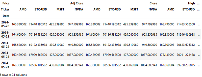

Descriptive Summary Statistics

Examining descriptive summary statistics of the Close price

df['Close'].describe().T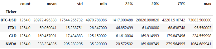

Descriptive summary statistics of the Close price

Analyzing standard deviation (std) of Close

df['Close'].std()
Ticker
AMD           37.437793
BTC-USD    17544.265732
MSFT          76.597961
NVDA         205.283295
dtype: float64

Standard deviation is the statistical measure of market volatility, measuring how widely prices are dispersed from the average price. If prices trade in a narrow trading range, the standard deviation will return a low value that indicates low volatility. Conversely, if prices swing wildly up and down, then standard deviation returns a high value that indicates high volatility.
Analyzing kurtosis (kurt) of Close

df['Close'].kurt()
Ticker
AMD        0.153687
BTC-USD   -0.706754
MSFT      -0.613576
NVDA       3.033257
dtype: float64

Kurtosis measures the degree of a distribution expressed as fat tails. Most of the investors are risk-averse which means that they prefer a distribution with low kurtosis, or we can explain differently as returns that are not far away from the mean.
Analyzing skewness (skew) of Close

df['Close'].skew()

Ticker
AMD        0.531194
BTC-USD    0.549099
MSFT       0.189534
NVDA       1.804376
dtype: float64

Skewness is the degree of asymmetry observed in a probability distribution. When data points on a bell curve are not distributed symmetrically to the left and right sides of the median, the bell curve is skewed. Distributions can be positive and right-skewed, or negative and left-skewed. A normal distribution exhibits zero skewness.
The positive skewness of a distribution indicates that an investor may expect frequent small losses and a few large gains from the investment.

Exploratory Data Analysis (EDA)

Plotting the stock Close price

plt.figure(figsize=(10,6))
df['Close','NVDA'].plot()
plt.title('NVDA Close Price USD')
plt.grid()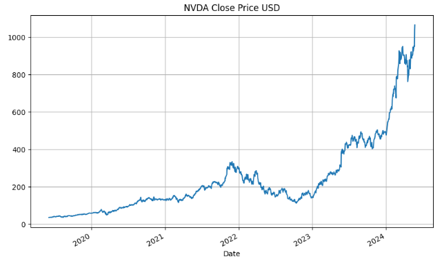

plt.figure(figsize=(10,6))
df['Close','BTC-USD'].plot()
plt.title('BTC-USD Close Price')
plt.grid()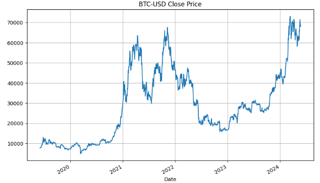

plt.figure(figsize=(10,6))
df['Close','AMD'].plot()
plt.title('AMD Close Price')
plt.grid()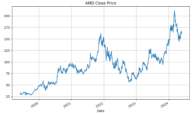

plt.figure(figsize=(10,6))
df['Close','MSFT'].plot()
plt.title('MSFT Close Price')
plt.grid()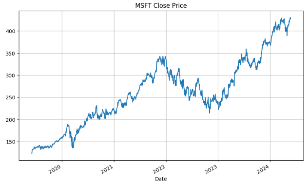

Plotting the stock correlation matrix

# checking correlation using heatmap

#plotting the heatmap for correlation
ax = sns.heatmap(df['Close'].corr(), annot=True)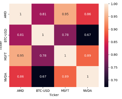

The correlation table is a two-dimensional matrix that shows the correlation coefficient between pairs of securities. The cells in the table are color-coded to highlight significantly positive and negative relationships.
Highly Positive Correlation Matchups: AMD — (NVDA, MSFT, BTC-USD), NVDA-MSFT, and BTC-MSFT.
Scaled covariance matrix

ax = sns.heatmap(df['Close'].cov()/1e6, annot=True)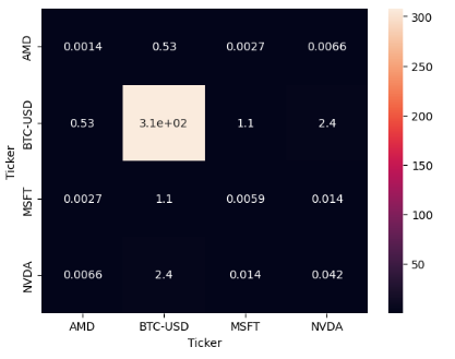

Covariance matrix and portfolio variance are essential tools that provide insights into the relationships between assets and help measure and manage portfolio risk.

Log Returns & Moving Average

Calculating log returns and SMA with the optimal length moav=47 (after scanning over a range of moav=10–50)

# Finding the log returns
stock_df['LogReturns'] = stock_df['Adj Close'].apply(np.log).diff().dropna()

# Using Moving averages
moav=47
stock_df['MovAvg'] = stock_df['Adj Close'].rolling(moav).mean().dropna()

# Logarithmic scaling of the data and rounding the result
stock_df['Log'] = stock_df['MovAvg'].apply(np.log).apply(lambda x: round(x, 2))

Plotting the Stock Log Returns %

plt.figure(figsize=(10,6))
stock_df['LogReturns'].plot()
plt.title('Stock Log Returns %')
plt.grid()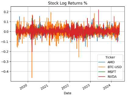

AutoARIMA Model Training & Forecasting

Setting the optimized input parameters and creating a DataFrame for predictions

# Days in the past to train on
days_to_train = 180

# Days in the future to predict
days_to_predict = 5

# Establishing a new DF for predictions
stock_df['Predictions'] = pd.DataFrame(index=stock_df['Log'].index,
                                       columns=stock_df['Log'].columns)

AutoARIMA Model Training

# Iterate through each stock
for stock in tqdm(stocks):
    
    # Current predicted value
    pred_val = 0
    
    # Training the model in a predetermined date range
    for day in tqdm(range(1000, 
                          stock_df['Log'].shape[0]-days_to_predict)):        

        # Data to use, containing a specific amount of days
        training = stock_df['Log'][stock].iloc[day-days_to_train:day+1].dropna()
        
        # Determining if the actual value crossed the predicted value
        cross = ((training.iloc[-1] >= pred_val >= training.iloc[-2]) or 
                 (training.iloc[-1] <= pred_val <= training.iloc[-2]))
        
        # Running the model when the latest training value crosses the predicted value or every other day 
        if cross or day % 2 == 0:

            # Finding the best parameters
            model    = AutoARIMA(start_p=0, start_q=0,
                                 start_P=0, start_Q=0,
                                 max_p=8, max_q=8,
                                 max_P=5, max_Q=5,
                                 error_action='ignore',
                                 information_criterion='bic',
                                 suppress_warnings=True)

AutoARIMA Model Forecasting

   # Getting predictions for the optimum parameters by fitting to the training set            
            forecast = model.fit_predict(training,
                                         n_periods=days_to_predict)

            # Getting the last predicted value from the next N days
            stock_df['Predictions'][stock].iloc[day:day+days_to_predict] = np.exp(forecast.iloc[-1])


            # Updating the current predicted value
            pred_val = forecast.iloc[-1]

# Shift ahead by 1 to compare the actual values to the predictions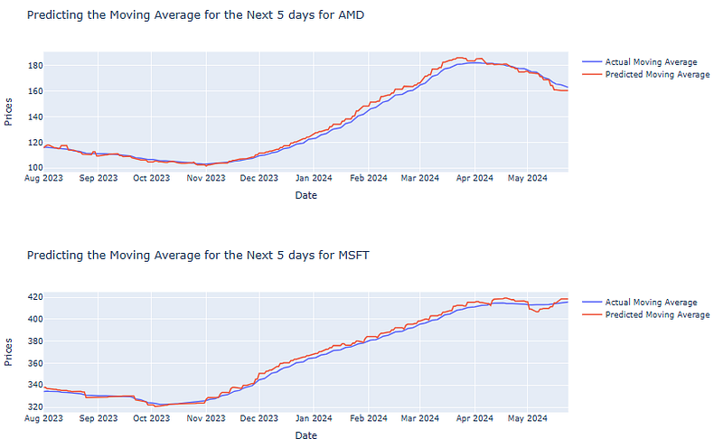
pred_df = stock_df['Predictions'].shift(1).astype(float).dropna()

Plotting Actual vs ARIMA Predicted Moving Average

for stock in stocks:
    
    fig = go.Figure()
    
    # Plotting the actual values
    fig.add_trace(go.Scatter(x=pred_df.index,
                             y=stock_df['MovAvg'][stock].loc[pred_df.index],
                             name='Actual Moving Average',
                             mode='lines'))
    
    # Plotting the predicted values
    fig.add_trace(go.Scatter(x=pred_df.index,
                             y=pred_df[stock],
                             name='Predicted Moving Average',
                             mode='lines'))
    
    # Setting the labels
    fig.update_layout(title=f'Predicting the Moving Average for the Next {days_to_predict} days for {stock}',
                      xaxis_title='Date',
                      yaxis_title='Prices')
    
    fig.show()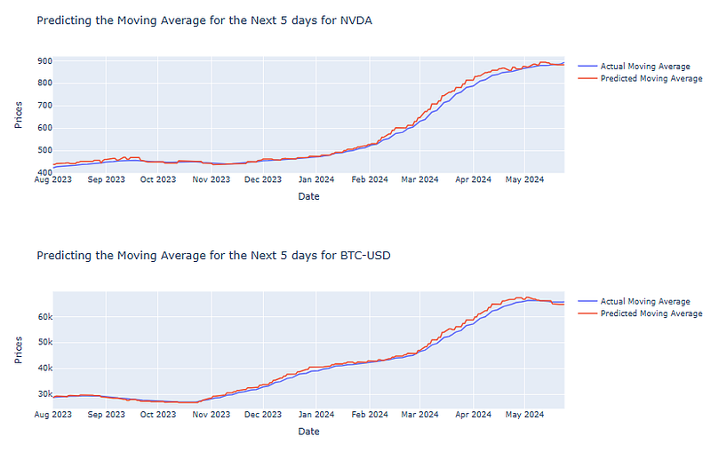

Actual vs ARIMA Predicted Moving Average: NVDA & BTC-USD

Actual vs ARIMA Predicted Moving Average: AMD & MSFT

Asset-Based Model Evaluation

Calculating RMSE for each stock

for stock in stocks:

    # Finding the root mean squared error
    rmse = mean_squared_error(stock_df['MovAvg'][stock].loc[pred_df.index], pred_df
[stock], squared=False)
    print(f"On average, the model is off by {rmse} for {stock}\n")

On average, the model is off by 13.973533904045606 for NVDA

On average, the model is off by 1046.8465603864092 for BTC-USD

On average, the model is off by 2.617724183009069 for AMD

On average, the model is off by 2.9525237555709047 for MSFT

Get Buy-Sell-Hold Positions

Let’s formulate our SMA strategy:
Buy — When the predicted price target shows a significant increase from the current price.
Sell — When the predicted price target shows a significant decrease from the current price.
Hold (or Do Nothing) — If the price target shows neither a significant increase or decrease from the current price.

def get_positions(difference, thres=3, short=True):
    """
    Compares the percentage difference between actual 
    values and the respective predictions.
    
    Returns the decision or positions to long or short 
    based on the difference.
    
    Optional: shorting in addition to buying
    """
    
    if difference > thres/100:
        
        return 1
    
    
    elif short and difference < -thres/100:
        
        return -1
    
    
    else:
        
        return 0

Preparing the DataFrame trade_df for our trading strategy

# Creating a DF dictionary for trading the model
trade_df = {}

# Getting the percentage difference between the predictions and the actual values
trade_df['PercentDiff'] = (stock_df['Predictions'].dropna() / 
                           stock_df['MovAvg'].loc[stock_df['Predictions'].dropna().index]) - 1

# Getting positions
trade_df['Positions'] = trade_df['PercentDiff'].map(lambda x: get_positions(x, 
                                                                                 thres=1, 
                                                                                 short=True) / len(stocks))

# Preventing lookahead bias by shifting the positions
trade_df['Positions'] = trade_df['Positions'].shift(2).dropna()

# Getting Log Returns
trade_df['LogReturns'] = stock_df['LogReturns'].loc[trade_df['Positions'].index]

Plotting Expected Stock Returns %

plt.figure(figsize=(10,6))
trade_df['PercentDiff'].plot()
plt.title('Stock Returns %')
plt.grid()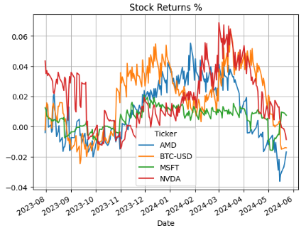

Plotting Stock Positions

plt.figure(figsize=(10,6))
trade_df['Positions'].plot()
plt.title('Stock Positions')
plt.grid()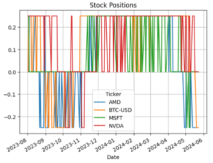

Plotting Stock Log Returns

plt.figure(figsize=(10,6))
trade_df['LogReturns'].plot()
plt.title('Stock Log Returns')
plt.grid()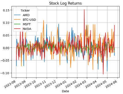

Plotting cumulative returns per stock using ARIMA forecast

# Calculating Returns by multiplying the 
# positions by the log returns
returns = trade_df['Positions'] * trade_df['LogReturns']

# Calculating the performance as we take the cumulative 
# sum of the returns and transform the values back to normal
performance = returns.cumsum().apply(np.exp)

# Plotting the performance per stock
px.line(performance,
        x=performance.index,
        y=performance.columns,
        title='Returns Per Stock Using ARIMA Forecast',
        labels={'variable':'Stocks',
                'value':'Returns'})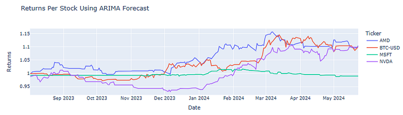

It might be a good idea to exclude the underperforming MSFT stock from the proposed tech portfolio.

SPY vs ARIMA Overall Portfolio Returns

Comparing the total cumulative portfolio returns against the SPY benchmark

# Returns for the portfolio
returns = (trade_df['Positions'] * trade_df['LogReturns']).sum(axis=1)

# Returns for SPY
spy = yf.download('SPY', start=returns.index[0]).loc[returns.index]

spy = spy['Adj Close'].apply(np.log).diff().dropna().cumsum().apply(np.exp)

# Calculating the performance as we take the cumulative sum of the returns and transform the values back to normal
performance = returns.cumsum().apply(np.exp)

# Plotting the comparison between SPY returns and ARIMA returns
fig = go.Figure()

fig.add_trace(go.Scatter(x=spy.index,
                         y=spy,
                         name='SPY Returns',
                         mode='lines'))

fig.add_trace(go.Scatter(x=performance.index,
                         y=performance.values,
                         name='ARIMA Returns on Portfolio',
                         mode='lines'))

fig.update_layout(title='SPY vs ARIMA Overall Portfolio Returns',
                  xaxis_title='Date',
                  yaxis_title='Returns')

fig.show()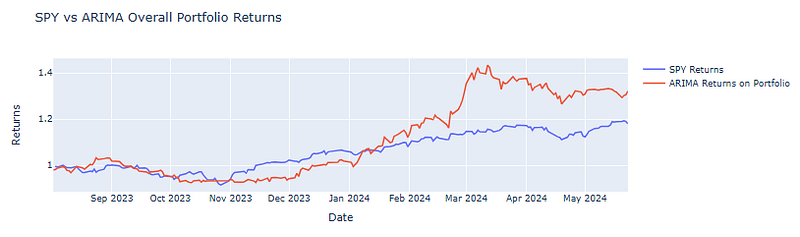

SPY Returns vs ARIMA Returns on Portfolio

It is clear that the ARIMA model outperforms SPY in 2024.

Conclusions

In this article, we have implemented and tested the vectorized backtesting & parameter tuning of AutoARIMA SMA trading strategy.
Our portfolio combines BTC-USD with 3 tech stocks (NVDA, AMD, and MSFT).
The backtesting strategy has been tested over a range of different SMA lengths and ARIMA parameter combinations to find the optimal set of parameters that maximize the expected return and outperforms the SPY benchmark.
We have shown how the ARIMA SMA trading model can take into account the relationship between an observation and its lagged values, allowing traders to assess how past price movements impact future movements.

Vectorized Backtesting & Parameter Tuning of AutoARIMA SMA Strategy: BTC-Tech vs S&P 500

Basic Settings, Imports & Installations

Input Historical Time Series Data

Descriptive Summary Statistics

Exploratory Data Analysis (EDA)

Log Returns & Moving Average

AutoARIMA Model Training & Forecasting

Asset-Based Model Evaluation

Get Buy-Sell-Hold Positions

SPY vs ARIMA Overall Portfolio Returns

Conclusions

Explore More

References

Contacts