
ML Classification Algorithms to Predict Market Movements and Backtesting
In this article, we will use the stock trading strategies based on multiple machine learning classification algorithms to predict the market movement. To analyze the performance we will perform simple vectorized backtesting and then test the best performing strategy using Backtrader to get a more realistic picture. You can find the relevant Jupyter notebook used in this article on my Github page. The overall approach is as follows:
- Gathering Historical Pricing Data.
- Feature Engineering.
- Build and Apply Classification Machine Learning Algorithms.
- Backtesting of Selected Strategy using Backtrader.
- Performance Analysis of Backtesting.
Gathering Historical Pricing Data
We are going to use the Nifty-50 index for this analysis. We will download the daily closing pricing data with the help of yfinance python library, calculate daily log returns, and derive market direction based on that. We will visualize the closing prices and daily returns to quickly check our data. Let’s go through the code:
# make the necessary imports
import numpy as np
from matplotlib import pyplot as plt
import pandas as pd
import seaborn as sns
import yfinance as yf
import warnings
from sklearn import linear_model
from sklearn.naive_bayes import GaussianNB
from sklearn.svm import SVC
from sklearn.ensemble import RandomForestClassifier
from sklearn.neural_network import MLPClassifier
import datetime
import pyfolio as pf
import backtrader as bt
from backtrader.feeds import PandasData
import warnings
# set the style and ignore warnings
plt.style.use(‘seaborn-colorblind’)
warnings.simplefilter(action=’ignore’, category=FutureWarning)
warnings.filterwarnings(‘ignore’)# this is to display images in notebook
%matplotlib inline
%config InlineBackend.figure_format = 'retina'# ticker and the start and end dates for testing
ticker = '^NSEI' # Nifty 50 benchmark
start = datetime.datetime(2010, 1, 1)
end = datetime.datetime(2020, 7, 31)# download ticker ‘Adj Close’ price from yahoo finance
stock = yf.download(ticker, progress=True, actions=True,start=start, end=end)['Adj Close']
stock = pd.DataFrame(stock)
stock.rename(columns = {'Adj Close':ticker}, inplace=True)
stock.head(2)# calculate daily log returns and market direction
stock['returns'] = np.log(stock / stock.shift(1))
stock.dropna(inplace=True)
stock['direction'] = np.sign(stock['returns']).astype(int)
stock.head(3)# visualize the closing price and daily returns
fig, ax = plt.subplots(2, 1, sharex=True, figsize = (12,6))
ax[0].plot(stock[ticker], label = f'{ticker} Adj Close')
ax[0].set(title = f'{ticker} Closing Price', ylabel = 'Price')
ax[0].grid(True)
ax[0].legend()ax[1].plot(stock['returns'], label = 'Daily Returns')
ax[1].set(title = f'{ticker} Daily Retunrs', ylabel = 'Returns')
ax[1].grid(True)
plt.legend()plt.tight_layout();
plt.savefig('images/chart1', dpi=300)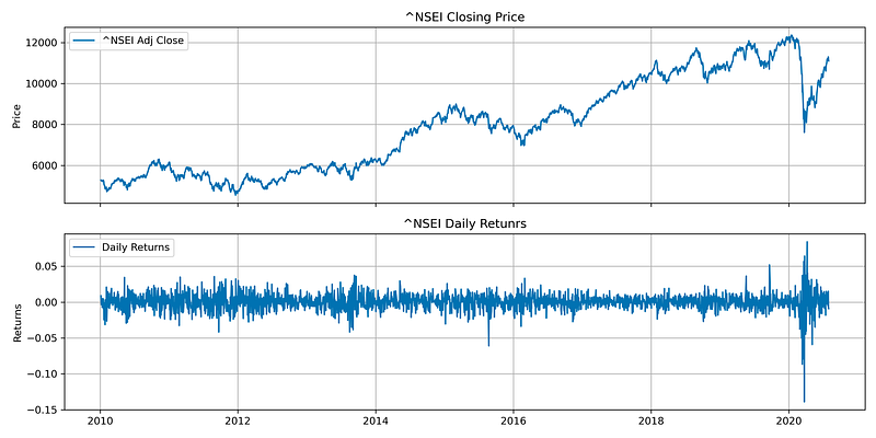
Code commentary:
- Make the necessary imports.
- Set the ticker as index Nifty-50 with start and end dates as 2010–01–01 and 2020–07–31.
- Download daily
Adj Closedata with the help ofyfinancefrom Yahoo Finance. - Calculate daily log returns and market direction using
np.sign().astype(int). - Visualize daily closing prices and log returns.
Feature Engineering
In this section, we will create feature variables to predict the market direction. As a first step, we will use five lags of the log-returns series and then digitize them as binary (0, 1) to predict the probability of an upward and a downward market movement as (+1, -1). The python code is as follows:
# define the number of lags
lags = [1, 2, 3, 4, 5]
# compute lagged log returns
cols = []
for lag in lags:
col = f'rtn_lag{lag}'
stock[col] = stock['returns'].shift(lag)
cols.append(col)stock.dropna(inplace=True)
stock.head(2)# function to transform the lag returns to binary values (0,+1)
def create_bins(data, bins=[0]):
global cols_bin
cols_bin = []
for col in cols:
col_bin = col + '_bin'
data[col_bin] = np.digitize(data[col], bins=bins)
cols_bin.append(col_bin)create_bins(stock)
stock[cols+cols_bin].head(2)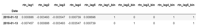
Code commentary:
- Compute five days lagged returns and shift the returns series to the number of lags to align them with one day forward return.
- Define the function to transform the lag returns to binary values (0,1) using the function
np.digitize().
Build and Apply Classification Machine Learning Algorithms
Now we are going to use Logistic regression, Gaussian Naive Bayes, Support Vector Machine (SVM), Random Forest, and MLP Classifier approach to predict the market direction as (+1, -1). Please refer to sklearn documentation for detail on these and other algorithms. We will then evaluate the performance of each of these models using vectorized backtesting and visualize the cumulative returns. Let’s go through the python code:
# create a dictionary of selected algorithms
models = {
 ‘log_reg’: linear_model.LogisticRegression(),
 ‘gauss_nb’: GaussianNB(),
 ‘svm’: SVC(),
 ‘random_forest’: RandomForestClassifier(max_depth=10, n_estimators=100),
 ‘MLP’ : MLPClassifier(max_iter=500),
}
# function that fits all models.
def fit_models(data):
mfit = {model: models[model].fit(data[cols_bin], data['direction']) for model in models.keys()}# function that predicts (derives all position values) from the fitted models
def derive_positions(data):
for model in models.keys():
data['pos_' + model] = models[model].predict(data[cols_bin])# function to evaluate all trading strategies
def evaluate_strats(data):
global strategy_rtn
strategy_rtn = []
for model in models.keys():
col = 'strategy_' + model
data[col] = data['pos_' + model] * data['returns']
strategy_rtn.append(col)
strategy_rtn.insert(0, 'returns')# fit the models
fit_models(stock)# derives all position values
derive_positions(stock)# evaluate all trading strategies by multiplying predicted directions to actual daily returns
evaluate_strats(stock)# calculate total return and std. deviation of each strategy
print('\nTotal Returns: \n')
print(stock[strategy_rtn].sum().apply(np.exp))
print('\nAnnual Volitility:')
stock[strategy_rtn].std() * 252 ** 0.5# number of trades over time for highest and second highest return strategy
print('Number of trades SVM = ', (stock['pos_svm'].diff()!=0).sum())
print('Number of trades Ramdom Forest = ',(stock['pos_random_forest'].diff()!=0).sum())# vectorized backtesting of the resulting trading strategies and visualize the performance over time
ax = stock[strategy_rtn].cumsum().apply(np.exp).plot(figsize=(12, 6),
title = 'Machine Learning Classifiers Return Comparison')
ax.set_ylabel("Cumulative Returns")
ax.grid(True);
plt.tight_layout();
plt.savefig('images/chart2', dpi=300)Code commentary:
- Create a dictionary of selected algorithms.
- Define a function that fits all models with
directioncolumn as the dependent variable and_bincolumns as feature variables. - Define a function that predicts all position values from the fitted models.
- Define a function to evaluate all trading strategies.
- Next, we fit the models, predict positions, and evaluate all trading strategies by multiplying predicted directions to actual daily returns.
- Calculate the total return and standard deviation of each strategy.
- Calculate the number of trades overtime for the highest and second-highest return strategies.
- Vectorize backtesting of the resulting trading strategies and visualize the performance over time.
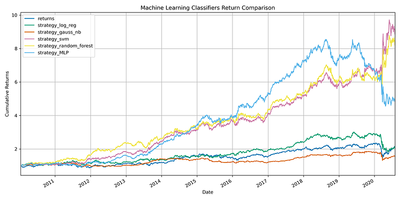
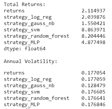
We can see that the support vector machine model has given the maximum total returns over time with comparable annual volatility with other models. However, it will be quite immature to deploy any such strategy based on vectorized backtesting results. Some of the reason are listed below:
- The number of trades is quite high and vectorized backtesting doesn’t account for costs such as trading and market slippage.
- The strategy accounts for both long and short positions however short selling may not be feasible due to multiple reasons.
Hence, our backtesting needs to be more realistic and event-driven to address the above gaps.
Backtesting of Selected Strategy using Backtrader
In this section, we will take our best performing model, i.e. support vector machine (SVM), and perform the backtesting using the python library Backtrader. The backtesting strategy will be as follows:
- We start with the initial capital of 100, 000 and trading commission as 0.1%.
- We buy when the
predictedvalue is +1 and sell (only if stock is in possession) when the predicted value is -1. - All-in strategy — when creating a buy order, buy as many shares as possible.
- Short selling is not allowed.
Let’s go through the python code:
# fetch the daily pricing data from yahoo finance
prices = yf.download(ticker, progress=True, actions=True, start=start, end=end)
prices.head(2)
# rename the columns as needed for Backtrader
prices.drop(['Close','Dividends','Stock Splits'], inplace=True, axis=1)
prices.rename(columns = {'Open':'open','High':'high','Low':'low','Adj Close':'close','Volume':'volume',
}, inplace=True)
prices.head(3)# add the predicted column to prices dataframe. This will be used as signal for buy or sell
predictions = stock['strategy_svm']
predictions = pd.DataFrame(predictions)
predictions.rename(columns = {'strategy_svm':'predicted'}, inplace=True)
prices = predictions.join(prices, how='right').dropna()
prices.head(2)OHLCV = ['open', 'high', 'low', 'close', 'volume']# class to define the columns we will provide
class SignalData(PandasData):
"""
Define pandas DataFrame structure
"""
cols = OHLCV + ['predicted']# create lines
lines = tuple(cols)# define parameters
params = {c: -1 for c in cols}
params.update({'datetime': None})
params = tuple(params.items())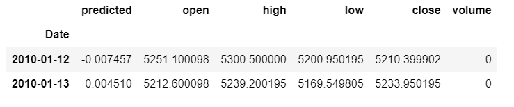
Code commentary:
- Fetch the daily pricing data from yahoo finance and rename the columns as OHLCV format needed for Backtrader.
- Take the SVM strategy returns from the
stockdataframe and join it to thepricesdataframe. This column’s value will be a signal to buy or sell while placing the order. - Define a custom
SignalDataclass for dataframe columns to be fed to Backtrader.
Now, we define the MLStrategy class for the backtesting strategy. It needs to be inherited from bt.Strategy. As we have predicted the market direction on the day’s closing price, hence we will use cheat_on_open=True when creating the bt.Cerebro object. This means the number of shares we want to buy will be based on day t+1’s open price. As a result, we also define the next_open method instead of next within the Strategy class.
# define backtesting strategy class
class MLStrategy(bt.Strategy):
    params = dict(
    )

    def __init__(self):
        # keep track of open, close prices and predicted value in the series
        self.data_predicted = self.datas[0].predicted
        self.data_open = self.datas[0].open
        self.data_close = self.datas[0].close

        # keep track of pending orders/buy price/buy commission
        self.order = None
        self.price = None
        self.comm = None
# logging function
def log(self, txt):
'''Logging function'''
dt = self.datas[0].datetime.date(0).isoformat()
print(f'{dt}, {txt}') def notify_order(self, order):
if order.status in [order.Submitted, order.Accepted]:
# order already submitted/accepted - no action required
return # report executed order
if order.status in [order.Completed]:
if order.isbuy():
self.log(f'BUY EXECUTED --- Price: {order.executed.price:.2f}, Cost: {order.executed.value:.2f},Commission: {order.executed.comm:.2f}'
)
self.price = order.executed.price
self.comm = order.executed.comm
else:
self.log(f'SELL EXECUTED --- Price: {order.executed.price:.2f}, Cost: {order.executed.value:.2f},Commission: {order.executed.comm:.2f}'
) # report failed order
elif order.status in [order.Canceled, order.Margin,
order.Rejected]:
self.log('Order Failed') # set no pending order
self.order = None def notify_trade(self, trade):
if not trade.isclosed:
return
self.log(f'OPERATION RESULT --- Gross: {trade.pnl:.2f}, Net: {trade.pnlcomm:.2f}') # We have set cheat_on_open = True.This means that we calculated the signals on day t's close price,
# but calculated the number of shares we wanted to buy based on day t+1's open price.
def next_open(self):
if not self.position:
if self.data_predicted > 0:
# calculate the max number of shares ('all-in')
size = int(self.broker.getcash() / self.datas[0].open)
# buy order
self.log(f'BUY CREATED --- Size: {size}, Cash: {self.broker.getcash():.2f}, Open: {self.data_open[0]}, Close: {self.data_close[0]}')
self.buy(size=size)
else:
if self.data_predicted < 0:
# sell order
self.log(f'SELL CREATED --- Size: {self.position.size}')
self.sell(size=self.position.size)Code commentary:
- The function
__init__tracks open, close, predicted, and pending orders. - The function
notify_ordertracks the order status. - The function
notify_tradeis triggered if the order is complete and logs profit and loss for the trade. - The function
next_openchecks the available cash and calculates the maximum number of shares that can be bought. It places the buy order if we don’t hold any position and thepredictedvalue is greater than zero. Else, it places the sell order if thepredictedvalue is less than zero.
Next, we instantiate SignalData and Cerebro objects and add prices dataframe, MLStrategy, initial capital, commission, and pyfolio analyzer. Finally, we run the backtest and capture the results.
# instantiate SignalData class
data = SignalData(dataname=prices)
# instantiate Cerebro, add strategy, data, initial cash, commission and pyfolio for performance analysis
cerebro = bt.Cerebro(stdstats = False, cheat_on_open=True)
cerebro.addstrategy(MLStrategy)
cerebro.adddata(data, name=ticker)
cerebro.broker.setcash(100000.0)
cerebro.broker.setcommission(commission=0.001)
cerebro.addanalyzer(bt.analyzers.PyFolio, _name='pyfolio')# run the backtest
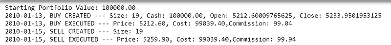
print('Starting Portfolio Value: %.2f' % cerebro.broker.getvalue())
backtest_result = cerebro.run()
print('Final Portfolio Value: %.2f' % cerebro.broker.getvalue())
Performance Analysis of Backtesting
We will analyze the performance statistics using pyfolio . pyfolio is a Python library for performance and risk analysis of financial portfolios developed by Quantopian Inc.
# Extract inputs for pyfolio
strat = backtest_result[0]
pyfoliozer = strat.analyzers.getbyname(‘pyfolio’)
returns, positions, transactions, gross_lev = pyfoliozer.get_pf_items()
returns.name = ‘Strategy’
returns.head(2)
# get benchmark returns
benchmark_rets= stock['returns']
benchmark_rets.index = benchmark_rets.index.tz_localize('UTC')
benchmark_rets = benchmark_rets.filter(returns.index)
benchmark_rets.name = 'Nifty-50'
benchmark_rets.head(2)# get performance statistics for strategy
pf.show_perf_stats(returns)# plot performance for strategy vs benchmark
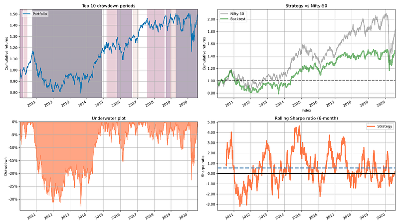
fig, ax = plt.subplots(nrows=2, ncols=2, figsize=(16, 9),constrained_layout=True)
axes = ax.flatten()pf.plot_drawdown_periods(returns=returns, ax=axes[0])
axes[0].grid(True)
pf.plot_rolling_returns(returns=returns,
factor_returns=benchmark_rets,
ax=axes[1], title='Strategy vs Nifty-50')
axes[1].grid(True)
pf.plot_drawdown_underwater(returns=returns, ax=axes[2])
axes[2].grid(True)
pf.plot_rolling_sharpe(returns=returns, ax=axes[3])
axes[3].grid(True)
# fig.suptitle('Strategy vs Nifty-50 (Buy and Hold)', fontsize=16, y=0.990)plt.grid(True)
plt.legend()
plt.tight_layout()
plt.savefig('images/chart3', dpi=300)Code commentary:
- We extract inputs needed for pyfolio from the backtesting result.
- Get the benchmark daily returns to compare and contrast with the strategy.
- Get performance statistics for the strategy using pyfolio
show_perf_stats. - Visualize drawdowns, cumulative returns, underwater plot, and rolling Sharpe ratio.
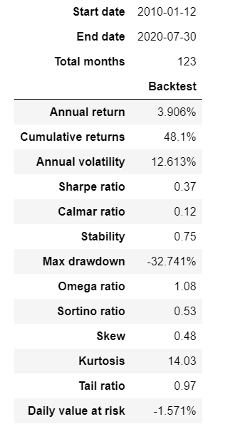
Let’s analyze the performance of our strategy. The annual return is just 3.9% and the cumulative return is 48% as compared to 8.86 times total return we observed during vectorized backtesting. If we visualize a few other performance parameters in comparison to the benchmark, we can see our strategy is not able to beat the performance of the simple buy and hold strategy.
So the obvious question is why? This is due to the fact that we paid a huge commission for a high number of trades. The second reason; we allowed no short selling while performing backtesting with Backtrader.
In conclusion, often the vectorized backtesting results may look great on paper however we need to consider all aspects of implementation shortfall and feasibility before we decide to implement such a strategy. Also, keep in mind that the capital market is not just about machine learning otherwise all data scientists would have become super-rich by now.
Happy investing and do leave your comments on the article!
Please Note: This analysis is only for educational purposes and the author is not liable for any of your investment decisions.
References:
- Python for Finance 2e: Mastering Data-Driven Finance by Yves Hilpisch
- Python for Finance Cookbook: Over 50 recipes for applying modern Python libraries to financial data analysis by Eryk Lewinson
- Machine Learning for Algorithmic Trading by Stefan Jansen
- Please check out my other articles/ posts on quantitative finance at my Linkedin page or on Medium.


