LSTM Model Prediction for the Trading Strategy

Introduction

The prediction of stock movements has long been a keen interest among financial experts, demanding significant computational power to handle and interpret various factors influencing the stock market. In our coursework, we delved into the application of neural networks, specifically Long Short-Term Memory (LSTM) models in time series analysis. We chose LSTM as our predicting model since it excels in capturing nonlinear relationships and patterns in time series data compared to traditional models.

This time, our project aims to devise stock trading strategies beyond simple price forecasts. We strive to predict specific trading actions — buy, hold, or sell — for each trading day. This approach enables the model to inform trading decisions directly, reducing the need for manual interpretation following price predictions. Such a model, if successful, could lessen the dependence on human judgment in stock trading. Nevertheless, crafting a strategy that is both consistently profitable and able to outperform the market presents a formidable challenge.

Data Preparation

Data Collection

All the data for our project is sourced directly from Bloomberg Terminal, encompassing both macroeconomic indicators and individual stock data:

Macroeconomic Indicators:

• Consumer Confidence Index (CCI)
• Unemployment Rate
• GDP Percentage Change
• Volatility Index (VIX)
• Retail Sales
• US Import Price Index by End Use All (MoM)
• US Export Price Index by End Use All (MoM)
• Personal Consumption Expenditure (PCE)
• Purchasing Managers’ Index (PMI)
• S&P 500 Index
• Nasdaq Index

Individual Stock Data:

• Companies: Synopsys (SPNS), IBM (IBM), Microsoft (MSFT)
• Stock Metrics: Open Price, High Price, Low Price, Close Price, and Volume

Some of the macroeconomic indicators are reported on a monthly or quarterly basis. To utilize these indicators for daily analysis, we interpolate their values to represent each day within the respective period.

After completing the data-cleaning process, our dataset comprises 7,925 observations. The time range spans from Jun. 13, 1992, to Nov. 28, 2023.

Trading Strategy

Building upon this dataset, we calculated various technical indicators, enhancing our analytical capabilities. The computed technical indicators included Moving Average Convergence Divergence (MACD), 14-Day Relative Strength Index (RSI14), 7-Day Relative Strength Index (RSI7), and Stochastic Oscillator K and D values. These technical indicators served as predictive features in our analysis.

In our project, we have also developed a systematic approach to generate a trading signal using MACD and RSI technical indicators. Here’s how it works:

• MACD signals

It was calculated by identifying changes in the sign of the MACD line. Based on these changes, signals are set to -1 (sell) or 1 (buy), with the most recent signal retained for continuity in data.

• RSI signals

We defined a function calculating RSI signals by analyzing the difference between the 7-day and 14-day RSI. It identifies crossover events used to generate buy or sell signals, with the latest signal carried forward when no new signal is developed.

• ‘signal_new’ trading strategy signals

We devised the ‘signal_new’ trading strategy using signals derived from the above. It is assigned as 1 (buy) or -1 (sell) only when both MACD and RSI signals suggest the same action. The most recent value is retained in the absence of signals, ensuring a consistent approach during signal gaps.

Feature Selection

We conducted feature selection by examining the correlation among the variables. We can easily see the associations between different features through the correlation matrix.

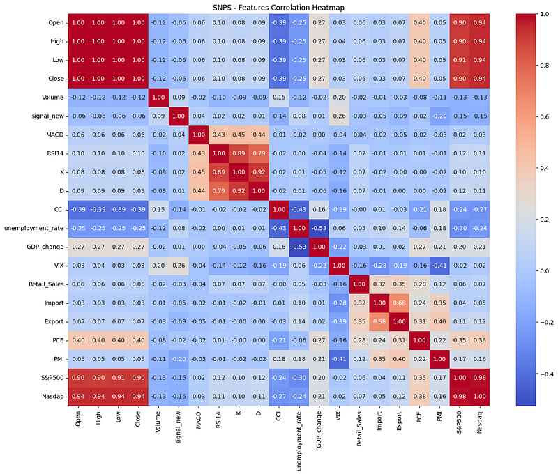
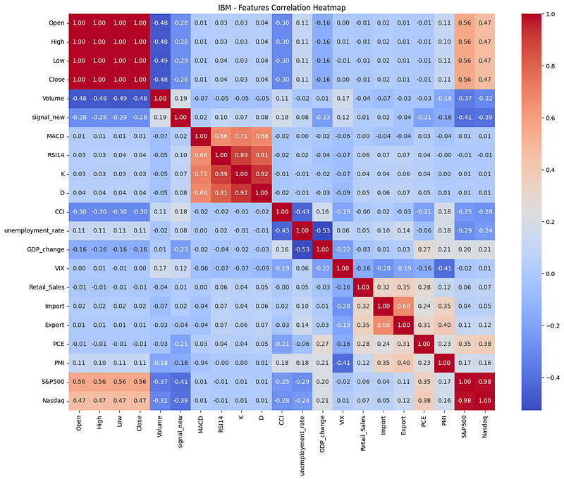
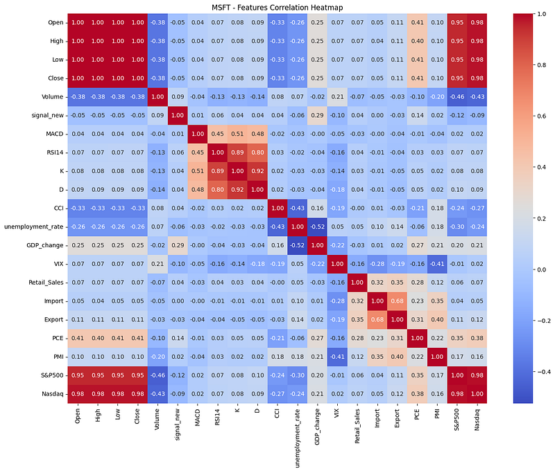
To ensure each feature effectively contributes to the prediction, we have excluded those with a correlation coefficient less than 0.015 from the target variable, retaining the remaining features for the LSTM model.

Subsequently, we split the dataset into training and testing sets, using 70% of the data for training purposes and 30% for testing. Additionally, we applied MinMaxScaler to normalize all features, scaling them within the range of 0 to 1. This preprocessing step ensures consistency in feature scales and contributes to the effectiveness of the modeling process.

Modeling

We built a LSTM model with 4 fully connected and 64 hidden layers. Each layer, except the output layer, is followed by a dropout rate of 0.35, which can be used to prevent overfitting. Also, we employed an alternative regularization technique with a 1e-5 weight decay value. Finally, we utilized the BCE Loss function and Adam optimizer for the classification problem and adaptive learning rate efficiency. We ran 200 epochs for training models for each company, and the results of the LSTM model-training process are shown below.

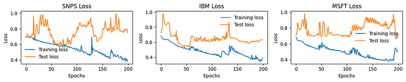
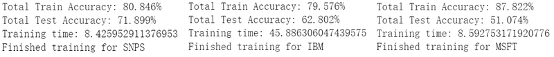
Overall, all 3 models reached approximately 80% of training accuracy, followed by 73.63%, 61.32%, and 53.35% testing accuracy. As for the losses, the training losses were observed by a decreasing trend over the epochs, indicating effective learning from the training data. The validation losses fluctuated, mostly reaching their lowest points around 50–100 epochs, except for MSFT’s model. This indicated that the models were still overfitting, so we added codes to save the best-performed (lowest training loss and validation loss) models while running epochs. Therefore, we could load the best model and make the predictions.

After the predictions, we used confusion matrices to evaluate the performance of the best model. The results are shown below.

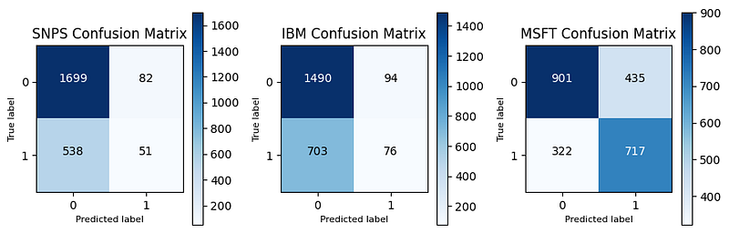
The accuracy rates for the 3 companies’ models were 75.02%, 71.35%, and 65.73%, respectively. As for the recall rates, they were 4.75%, 30.42%, and 48.22%. The model for SNPS had relatively high accuracy but a very low recall rate. This implied that while the model correctly predicted a large percentage of the total cases (both positive and negative), it was poor at identifying positive cases. In practical terms, the model may fail to detect when investors buy the stocks, but it’s good at correctly determining when to sell the stocks, which is more important to avoid the risk of drawdown. On the other hand, models for IBM and MSFT present a case with moderate accuracy and considerably higher recall compared to the SNPS’s model. This suggests that they are much more effective at identifying positive cases.

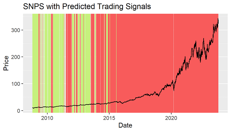
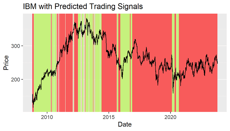
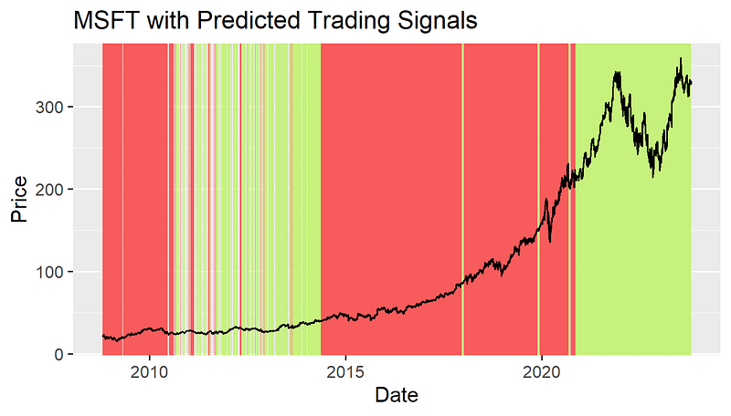
The graphs of the stock prices and the predicted trading signals for 3 companies are shown below. (Period: Oct. 22, 2008 — Oct. 22, 2023)

Backtesting Result of Predicted Trading Strategy

We output the previously predicted results into Excel and put them into R for the backtest. During the backtesting period, we would buy stocks when the trade signal first appeared as 1 and continue to hold them until a 0 appeared; at this point, we would sell the stocks and stay uninvested until the next occurrence of 1.

When comparing four investment strategies, we previously set trading signals consisting of MACD and RSI, LSTM model forecast signals, lump sum investing, and Dollar-Cost averaging. The total return rate, annualized return rate, and risk of the three stocks under these four investment strategies are calculated respectively, and the results are as follows.

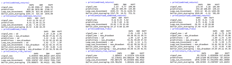
We conducted backtests on investment returns for three periods: the most extended period available in the database (since 1992), the past 20 years, and the past 15 years. When comparing our custom investment strategy and the trade signals predicted by the LSTM model, it is evident that trading based on the trade signals generated by the LSTM model results in a significantly higher total return rate for SNPS than the actual investment strategy. When calculating the return-risk ratio (total return rate / standard deviation), we obtain values of 93.78 and 149.17 from the past 15 years, indicating that the LSTM model allows investors to achieve a 149.17% return rate per unit of risk. In contrast, the backtest result for MSFT shows that the investment strategy based on the LSTM model yields lower returns than the actual strategy. This might be due to the low accuracy rate of the MSFT model, which affects its predictive performance.

Compared to our investment strategy defined by technical indicators, both lump-sum investment and dollar-cost averaging yield higher total returns. However, it is also evident from the risk metrics that they are accompanied by higher volatility in returns and maximum drawdown. This ultimately depends on the investor’s preference in choosing between these options.

Conclusion

The primary focus of this project was to determine whether the LSTM model could accurately identify buy and sell points according to our original strategy. The results are affirmative, with the model achieving about 70% accuracy. However, there were instances of overfitting, suggesting that future adjustments to the parameters could further improve accuracy. Trading based on the signals predicted by the model yielded higher investment returns than our original strategy. The reason lies in the model generating fewer trade signals during consolidation periods, thus avoiding the frequent buying and selling characteristic of our original strategy, which often led to reduced trading performance.