
Full-Fledged Technical Analysis of Top Growth Stocks: Backtesting Volatility Resilience vs Profitability
Backtesting a wide spectrum of algo trading strategies, addressing volatility resilience vs profitability, simulating VaR, and computing trend-following technical indicators of top growth stocks.
“Technical analysis is a skill that improves with experience and study. Always be a student, and keep learning.” — John J Murphy

- This article focuses on introducing some of the simple yet powerful techniques applied during technical analysis with Python for algorithmic trading (aka algo trading) of top growth stocks to watch.
- Technical Analysis is the basis for algo trading when you use software products to open and close trades according to set rules such as points of price movement in an underlying market. Once the current market conditions match any predetermined criteria, trading algorithms (algos) can execute a buy or sell order on your behalf.
- Technical analysis based algo trading analyzes historical price and volume data to identify patterns and trends. By using a combination of chart patterns, moving averages, oscillators, and other technical indicators, traders aim to forecast future price movements and make trading decisions.
Objectives
- Load stock historical stock data from the web.
- Use risk-aware technical analysis for algo-trading.
- Joint analysis of several technical indicators.
- Backtesting basic and mixed algo-trading strategies.
Contents
- The Sharpe Ratio of Top 7 Tech Stocks
- NVDA PSR & 95% CI
- NVDA Daily/Cumulative Returns
- NVDA Keltner Channel (KC) Strategy
- NVDA VWAP Support & Resistance
- NVDA Fundamental Analysis
- Backtesting NVDA Williams %R & MACD Trading Strategy
- Monte Carlo Simulation of NVDA Value-at-Risk (VaR)
- NVDA RSI & Bollinger Bands Support-Resistance
- Risk-Return Comparison of 10 Stocks to Watch
- Backtest GOOG RSI-SMA Trading Strategies
- AMD SMA-MACD-ADX Trend-Following Analysis
Let’s delve into the specifics of the proposed algorithmic trading methodology in Python.
The Sharpe Ratio of Top 7 Tech Stocks
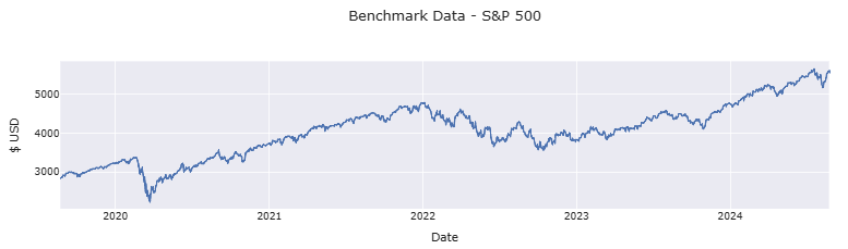
- Let’s look at the Sharpe Ratio (SR) [1] of top 7 tech stocks such as MSFT, AAPL, NVDA, META, GOOG, AMZN, and TSLA. Here, S&P 500 will be used as a benchmark rather than the risk-free interest rate.
- Typically, a SR of 1 or better is good, 2 or better is very good, and 3 or better is excellent [2].
- Importing libraries and loading the input stock and S&P 500 data in bulk
# Importing libraries
import yfinance as yf
import pandas as pd
import numpy as np
import plotly.io as pio
import plotly.express as px

# Set plot style
pio.templates.default = "seaborn"

# Loading stock data in bulk; keeping only dates with values across all ticker symbols
stock_data = yf.download('MSFT AAPL NVDA META GOOG AMZN TSLA', period='5Y').dropna()
benchmark_data = data = yf.download('^GSPC', period='5Y').dropna()

stock_data = stock_data['Close']
stock_data.tail()

icker       AAPL      AMZN        GOOG       META      MSFT        NVDA       TSLA
Date
2024-08-19 225.889999 178.220001 168.399994 529.280029 421.529999 130.000000 222.720001
2024-08-20 226.509995 178.880005 168.960007 526.729980 424.799988 127.250000 221.100006
2024-08-21 226.399994 180.110001 167.630005 535.159973 424.140015 128.500000 223.270004
2024-08-22 224.529999 176.130005 165.490005 531.929993 415.549988 123.739998 210.660004
2024-08-23 226.149994 176.964996 166.759995 531.090027 415.239990 128.009995 217.500000

benchmark_data = benchmark_data[['Close']].rename(columns={'Close':'S&P 500'})
benchmark_data.tail()

           S&P 500
Date
2024-08-19 5608.250000
2024-08-20 5597.120117
2024-08-21 5620.850098
2024-08-22 5570.640137
2024-08-23 5618.700195- Plotting the stock and S&P 500 Close price data
# Visualization of stock data
fig = px.line(stock_data,
              title='Stock Data',
              labels={'value':'$ USD',
                      'variable':'Ticker'})
fig.show()

# Visualization of benchmark data
fig = px.line(benchmark_data,
              title='Benchmark Data - S&P 500',
              labels={'value':'$ USD'})
fig.update_layout(showlegend=False)
fig.show()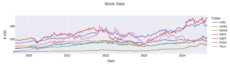
- Calculating and plotting the stock and benchmark daily returns
stock_returns = stock_data.pct_change()

fig = px.line(stock_returns,
              title='Stock % Change',
              labels={'variable':'Ticker'})
fig.show()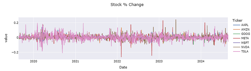
sp_returns = benchmark_data['S&P 500'].pct_change()

fig = px.line(sp_returns, title='S&P 500 % Change')
fig.update_layout(showlegend=False)
fig.show()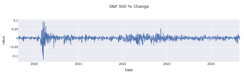
- Calculating and plotting the difference between stock and benchmark daily returns
excess_returns = stock_returns.sub(sp_returns, axis=0).dropna()

fig = px.line(excess_returns, labels={'variable':'Ticker'}, title='Excess Returns')
fig.show()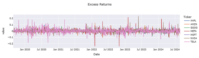
- Calculating the average of the above Excess Returns to plot the stock yields per day compared to S&P 500
avg_excess_return = excess_returns.mean()

fig = px.bar(avg_excess_return, color=avg_excess_return.index)
fig.update_layout(showlegend=False, title='Average Excess Returns')
fig.show()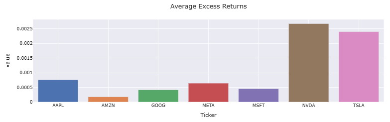
- Calculating STD of the Excess Returns to assess the amount of stock investment risk compared to S&P 500
sd_excess_return = excess_returns.std()

fig = px.bar(sd_excess_return, color=sd_excess_return.index)
fig.update_layout(showlegend=False, title='Standard Deviation of the Return Difference')
fig.show()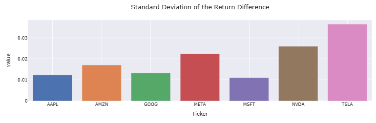
- Computing and plotting the annualized SR as the Average Excess Returns to STD of the Excess Returns ratio [1, 2]
daily_sharpe_ratio = avg_excess_return.div(sd_excess_return)

# annualized Sharpe ratio for trading days in a year (5 days, 52 weeks, no holidays)
annual_factor = np.sqrt(252)
annual_sharpe_ratio = daily_sharpe_ratio.mul(annual_factor)

fig = px.bar(annual_sharpe_ratio, color=annual_sharpe_ratio.index)
fig.update_layout(showlegend=False, title='Annualized Sharpe Ratio: Stocks vs S&P 500')
fig.show()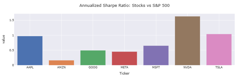
Inferences:
- AMZN, GOOG, META, and MSFT have SR<1.0. A ratio under 1.0 is considered sub-optimal.
- AAPL and TSLA have the SR values of 0.97 and 1.04, respectively. A SR of close to 1.0 or greater is typically considered good.
- NVDA has the SR of 1.63 that is higher than the other 6 tech stocks.
- In risk-adjusted terms, NVDA would be the most acceptable investment opportunity.
NVDA PSR & 95% CI
- Fetching the NVDA stock data 2022–2024 with twelvedata.com API [3]
# IMPORTING PACKAGES

import requests
import numpy as np
import matplotlib.pyplot as plt
import pandas as pd
from termcolor import colored as cl
from math import floor

plt.rcParams['figure.figsize'] = (12,6)
plt.style.use('fivethirtyeight')

# EXTRACTING STOCK DATA

def get_historical_data(symbol, start_date):
    api_key = 'YOUR API KEY'
    api_url = f'https://api.twelvedata.com/time_series?symbol={symbol}&interval=1day&outputsize=5000&apikey={api_key}'
    raw_df = requests.get(api_url).json()
    df = pd.DataFrame(raw_df['values']).iloc[::-1].set_index('datetime').astype(float)
    df = df[df.index >= start_date]
    df.index = pd.to_datetime(df.index)
    return df

intc = get_historical_data('NVDA', '2022-01-01')
intc.tail()

           open      high      low     close  volume
datetime
2024-08-19 124.28000 130.00000 123.42 130.00 318333600.0
2024-08-20 128.39999 129.88000 125.89 127.25 300087400.0
2024-08-21 127.32000 129.35001 126.66 128.50 257883600.0
2024-08-22 130.02000 130.75000 123.10 123.74 376189100.0
2024-08-23 125.86000 129.60001 125.22 129.37 322154200.0

intc.shape
(664, 5)- Plotting the NVDA Plotly candlesticks
import plotly.graph_objects as go

import pandas as pd
from datetime import datetime

df = intc.copy()

fig = go.Figure(data=[go.Candlestick(x=df.index,
                open=df['open'],
                high=df['high'],
                low=df['low'],
                close=df['close'])])

fig.show()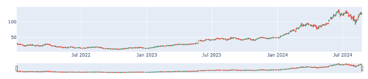
- Candlesticks are useful when trading as they show 4 price points (open, close, high, and low) throughout the period of interest. If the real body is green, it means the close was higher than the open. When the real body is red, it means the close was lower than the open. Emotion often dictates trading, which can be read in candlestick charts.
- Calculating the mean, skewness, and kurtosis of daily returns
prices=intc['close']
daily_return = prices.pct_change(1)
# Check the mean, skewness and kurtosis
print('- NVDA daily returns:')
print('Mean:', daily_return.mean())
print('Skewness:', daily_return.skew())
print('Kurtosis:', daily_return.kurtosis())

- NVDA daily returns:
Mean: 0.002827624633924218
Skewness: 0.7275340047117553
Kurtosis: 3.969024954729987- Calculating the NVDA Probabilistic Sharpe Ratio (PSR) with 95% Confidence Intervals (CI) [4, 5]
skew0=0.7275340047117553
kurt0=3.969024954729987

from scipy.stats import norm

# Estimated Sharpe Ratio (SR) and number of observations (N)
SR_hat = 1.63
N = 252

# Calculate Standard Deviation of Sharpe Ratio (Std Dev SR)
def standard_deviation_sharpe_ratio(sharpe_ratio, num_obs, skewness=0, kurtosis=3):
    """Estimates standard Deviation of Sharpe Ratio

    Parameters:
    - sharpe_ratio: Sharpe ratio of the strategy
    - bench_sharpe_ratio: Sharpe ratio of the benchmark
    - num_obs: Number of observations
    - skewness: Skewness of the strategy returns (default 0)
    - kurtosis: Kurtosis of the strategy returns (default 3)

    Returns:
    - std_dev: Standard Deviation of Sharpe Ratio
    """
    return np.sqrt(
        (1 - skewness*sharpe_ratio +
         (kurtosis-1)/4*sharpe_ratio**2
        ) / (num_obs-1)
    )

# Portfolio Returns with Normality
sigma_hat_normal_returns = standard_deviation_sharpe_ratio(sharpe_ratio=SR_hat,
                                                           num_obs=N,
                                                           skewness=skew0,
                                                           kurtosis=kurt0)

# Portfolio Returns with Non-Normality
sigma_hat_higher_moments = standard_deviation_sharpe_ratio(sharpe_ratio=SR_hat,
                                                           num_obs=N,
                                                           skewness=skew0,
                                                           kurtosis=kurt0)

def two_sided_confidence_intervals(sharpe_ratio, standard_deviation, confidence_level):
    """Sharpe Ratio two-sided confidence intervals

    Parameters:
    - sharpe_ratio: Sharpe ratio of the strategy
    - standard_devation: Standard Deviation of Sharpe Ratio
    - confidence_level: level of confidence (fraction: i.e. 0.90 for 90%)

    Returns:
    - lower_bound: two-sided lower bound
    - upper_bound: two-sided upper bound
    """
    # Two-sided (1-alpha)% Confidence Interval
    alpha = 1 - confidence_level
    Z_alpha_over_2 = norm.ppf(1-alpha/2)  # 95% CI

    lower_bound = sharpe_ratio - Z_alpha_over_2 * standard_deviation
    upper_bound= sharpe_ratio + Z_alpha_over_2 * standard_deviation

    return lower_bound, upper_bound

lower_norm, upper_norm = two_sided_confidence_intervals(SR_hat,
                                                  sigma_hat_normal_returns,
                                                  0.95)

lower_non_norm, upper_non_norm = two_sided_confidence_intervals(SR_hat,
                                                  sigma_hat_higher_moments,
                                                  0.95)

# Print the confidence intervals
print(f"Normally Distributed; Two-sided 95% CI:     [{lower_norm:2.4f}, {upper_norm:2.4f}]")
print(f"Non-Normally Distributed; Two-sided 95% CI: [{lower_non_norm:2.4f}, {upper_non_norm:2.4f}]")

Normally Distributed; Two-sided 95% CI:     [1.4647, 1.7953]
Non-Normally Distributed; Two-sided 95% CI: [1.4647, 1.7953]

def probabilistic_sharpe_ratio(sharpe_ratio, bench_sharpe_ratio, num_obs, skewness, kurtosis):
    """
    Calculates the Probabilistic Sharpe Ratio

    Parameters:
    - sharpe_ratio: Sharpe ratio of the strategy
    - bench_sharpe_ratio: Sharpe ratio of the benchmark
    - num_obs: Number of observations
    - skewness: Skewness of the strategy returns
    - kurtosis: Kurtosis of the strategy returns

    Returns:
    - psr: Probabilistic Sharpe Ratio
    """

    sr_diff = sharpe_ratio - bench_sharpe_ratio
    sr_vol = standard_deviation_sharpe_ratio(sharpe_ratio, num_obs, skewness, kurtosis)
    psr = norm.cdf(sr_diff / sr_vol)

    return psr

SR = 1.63  # Your strategy's Sharpe Ratio
Bench_SR = 0.65  # Benchmark Sharpe Ratio
#https://www.morningstar.com/indexes/spi/spx/risk
skewness = 0.72  # Skewness of your strategy
kurtosis = 3.97  # Kurtosis of your strategy
N = 252  # Number of observations (trading days in a year, for example)

#Skewness: 0.7275340047117553
#Kurtosis: 3.969024954729987

# Calculate PSR
PSR_value = probabilistic_sharpe_ratio(SR, Bench_SR, N, skewness, kurtosis)
print(f"Probabilistic Sharpe Ratio: {PSR_value}")

Probabilistic Sharpe Ratio: 1.0
Inferences:
- Combinations of skewness and kurtosis in returns distribution impact the STD and the confidence bands of the SR.
- The PSR metric accounts for the STD and uncertainty associated with estimating SR (Type I errors) [5].
NVDA Daily/Cumulative Returns
- Let’s continue using the NVDA stock dataset 2022–2024 intc, being referred to as DAT1.
- Plotting the DAT1 candlesticks and volume with mplfinance-module
!pip install mplfinance
import mplfinance as mpf
import pandas as pd
import numpy as np
import matplotlib.pyplot as plt

# Create a style with adjusted font size
style = mpf.make_mpf_style(base_mpl_style='default', rc={'font.size': 12})  # Set the font size here
# Create a new figure and set the title
fig, axes = mpf.plot(intc, type='candle', volume=True,
   title='NVDA Stock Price', ylabel='Price', ylabel_lower='Volume',
   show_nontrading=True, returnfig=True, style=style)
plt.style.use('dark_background')
# Retrieve the axis objects from the returned list
ax = axes[0]

# Customize the appearance of the plot
ax.grid(True)  # Display grid lines

# Save the plot to an image file
#fig.savefig('tesla_candlestick_chart.png')

# Show the plot on the screen
mpf.show()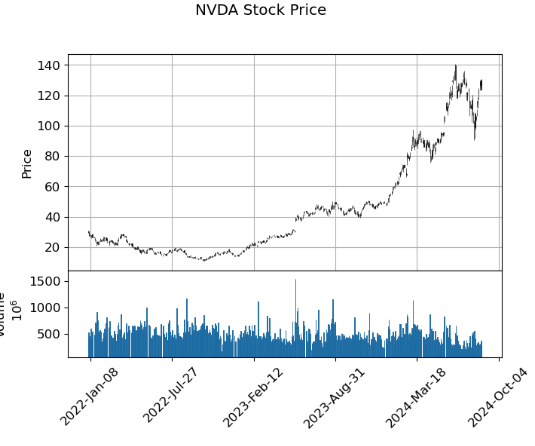
- We can see that the lower the trading volume, the skinnier the candlestick body. A higher-volume days result in wider candlestick. Here, we plot volume at the bottom of a price chart as a series of rectangles.
- Computing and plotting the stock daily returns
data=intc.copy()

# Convert 'volume' column to numeric, handle non-numeric values
data['volume'] = pd.to_numeric(data['volume'], errors='coerce')
non_numeric_values = data['volume'].isnull()
if non_numeric_values.any():
   data['volume'] = np.where(non_numeric_values, 0, data['volume'])

prices=intc['close']
daily_return = prices.pct_change(1)
daily_return.plot(title='NVDA Daily Returns',figsize=(12, 6))

# Check the mean, skewness and kurtosis
print('- NVDA daily returns:')
print('Mean:', daily_return.mean())
print('Skewness:', daily_return.skew())
print('Kurtosis:', daily_return.kurtosis())

- NVDA daily returns:
Mean: 0.002827624633924218
Skewness: 0.7275340047117553
Kurtosis: 3.969024954729987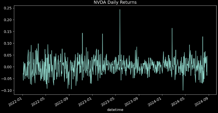
- Daily returns provide valuable insights into short-term performance, allow for meaningful comparisons, and help identify market trends.
- By analyzing the above daily returns, investors can gain insights into the overall direction of the market. For example, a series of consistently positive daily returns in the technology sector may indicate a bullish market sentiment for tech stocks.
- Computing and plotting the stock cumulative returns
cum_return = (1 + daily_return).cumprod() - 1
cum_return.plot(title='NVDA Cumulative Returns',figsize=(12, 6))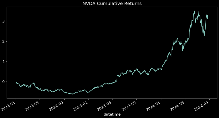
- Cumulative returns are the total gains or losses of an investment over a specific period. It is a crucial metric that investors use to determine the overall performance of their portfolio.
- This information can help investors adjust their portfolio to maximize their returns.
- However, taxes can substantially reduce the cumulative returns for most investments unless they are held in tax-advantaged accounts.
NVDA Keltner Channel (KC) Strategy
- In this section, the goal is to backtest the Keltner Channel (KC) indicator [3] that has 3 channel lines: middle line, upper line and lower line. The lines are calculated as follows [6]:
Upper line = EMA + (ATR x multiplier) Middle line = EMA Lower line = EMA — (ATR x multiplier)
- The slope of the channel denotes the price trend in the market. A rising channel implies that an uptrend is in place; a falling channel indicates a downtrend; whereas a flat or sideways channel implies a ranging market.
- Calculating the KC indicator for the DAT1 dataset [3]
# KELTNER CHANNEL CALCULATION

def get_kc(high, low, close, kc_lookback, multiplier, atr_lookback):
    tr1 = pd.DataFrame(high - low)
    tr2 = pd.DataFrame(abs(high - close.shift()))
    tr3 = pd.DataFrame(abs(low - close.shift()))
    frames = [tr1, tr2, tr3]
    tr = pd.concat(frames, axis = 1, join = 'inner').max(axis = 1)
    atr = tr.ewm(alpha = 1/atr_lookback).mean()

    kc_middle = close.ewm(kc_lookback).mean()
    kc_upper = close.ewm(kc_lookback).mean() + multiplier * atr
    kc_lower = close.ewm(kc_lookback).mean() - multiplier * atr

    return kc_middle, kc_upper, kc_lower
# kc_lookback, multiplier, atr_lookback  20, 2, 10
intc = intc.iloc[:,:4]
intc['kc_middle'], intc['kc_upper'], intc['kc_lower'] = get_kc(intc['high'], intc['low'], intc['close'], 20, 2, 20)
intc.tail()

           open      high      low    close  kc_middle  kc_upper   kc_lower
datetime
2024-08-19 124.28000 130.00000 123.42 130.00 115.434182 128.917605 101.950759
2024-08-20 128.39999 129.88000 125.89 127.25 115.996840 129.217092 102.776588
2024-08-21 127.32000 129.35001 126.66 128.50 116.592229 129.420469 103.763988
2024-08-22 130.02000 130.75000 123.10 123.74 116.932599 129.884427 103.980771
2024-08-23 125.86000 129.60001 125.22 129.37 117.524856 130.415094 104.634618- Implementing the KC trading strategy [3]
# KELTNER CHANNEL STRATEGY

def implement_kc_strategy(prices, kc_upper, kc_lower):
    buy_price = []
    sell_price = []
    kc_signal = []
    signal = 0

    for i in range(len(prices)):
        if prices.iloc[i] < kc_lower.iloc[i] and prices.iloc[i+1] > prices.iloc[i]:
            if signal != 1:
                buy_price.append(prices.iloc[i])
                sell_price.append(np.nan)
                signal = 1
                kc_signal.append(signal)
            else:
                buy_price.append(np.nan)
                sell_price.append(np.nan)
                kc_signal.append(0)
        elif prices.iloc[i] > kc_upper.iloc[i] and prices.iloc[i+1] < prices.iloc[i]:
            if signal != -1:
                buy_price.append(np.nan)
                sell_price.append(prices.iloc[i])
                signal = -1
                kc_signal.append(signal)
            else:
                buy_price.append(np.nan)
                sell_price.append(np.nan)
                kc_signal.append(0)
        else:
            buy_price.append(np.nan)
            sell_price.append(np.nan)
            kc_signal.append(0)

    return buy_price, sell_price, kc_signal

buy_price, sell_price, kc_signal = implement_kc_strategy(intc['close'], intc['kc_upper'], intc['kc_lower'])- Calculating and plotting the KC trading signals for the DAT1 dataset
# TRADING SIGNALS PLOT
plt.figure(figsize=(12,6))
plt.plot(intc['close'], linewidth = 2, label = 'NVDA')
plt.plot(intc['kc_upper'], linewidth = 2, color = 'orange', linestyle = '--', label = 'KC UPPER')
plt.plot(intc['kc_middle'], linewidth = 1.5, color = 'grey', label = 'KC MIDDLE')
plt.plot(intc['kc_lower'], linewidth = 2, color = 'orange', linestyle = '--', label = 'KC LOWER')
plt.plot(intc.index, buy_price, marker = '^', color = 'green', markersize = 15, linewidth = 0, label = 'BUY SIGNAL')
plt.plot(intc.index, sell_price, marker = 'v', color= 'r', markersize = 15, linewidth = 0, label = 'SELL SIGNAL')
plt.legend(loc = 'lower right')
plt.title('NVDA KELTNER CHANNEL 20/2/20 TRADING SIGNALS')
plt.show()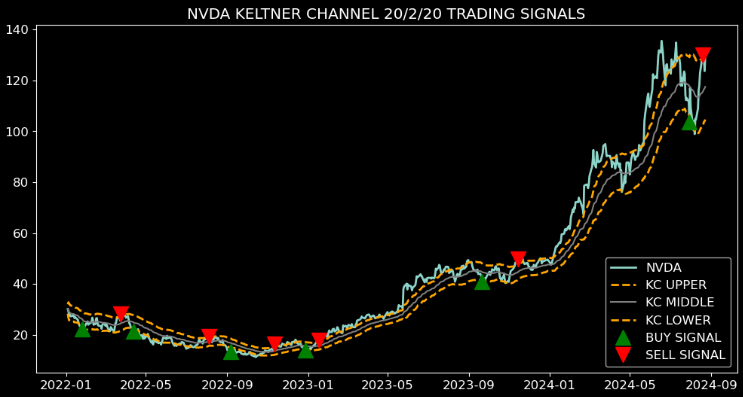
- Creating the stock position [3]
# STOCK POSITION

position = []
for i in range(len(kc_signal)):
    if kc_signal[i] > 1:
        position.append(0)
    else:
        position.append(1)

for i in range(len(intc['close'])):
    if kc_signal[i] == 1:
        position[i] = 1
    elif kc_signal[i] == -1:
        position[i] = 0
    else:
        position[i] = position[i-1]

close_price = intc['close']
kc_upper = intc['kc_upper']
kc_lower = intc['kc_lower']
kc_signal = pd.DataFrame(kc_signal).rename(columns = {0:'kc_signal'}).set_index(intc.index)
position = pd.DataFrame(position).rename(columns = {0:'kc_position'}).set_index(intc.index)

frames = [close_price, kc_upper, kc_lower, kc_signal, position]
strategy = pd.concat(frames, join = 'inner', axis = 1)

strategy

          close   kc_upper kc_lower kc_signal kc_position
datetime
2022-01-03 30.121 31.973000 28.269000 0 1
2022-01-04 29.290 32.770956 26.619776 0 1
2022-01-05 27.604 32.281595 25.646342 0 1
2022-01-06 28.178 31.916415 25.589327 0 1
2022-01-07 27.247 31.489336 25.353895 0 1
... ... ... ... ... ...
2024-08-19 130.000 128.917605 101.950759 -1 0
2024-08-20 127.250 129.217092 102.776588 0 0
2024-08-21 128.500 129.420469 103.763988 0 0
2024-08-22 123.740 129.884427 103.980771 0 0
2024-08-23 129.370 130.415094 104.634618 0 0
664 rows × 5 columns- Backtesting the above KC strategy [3] by investing $100k in NVDA
# BACKTESTING

intc_ret = pd.DataFrame(np.diff(intc['close'])).rename(columns = {0:'returns'})
kc_strategy_ret = []

for i in range(len(intc_ret)):
    returns = intc_ret['returns'][i]*strategy['kc_position'][i]
    kc_strategy_ret.append(returns)

kc_strategy_ret_df = pd.DataFrame(kc_strategy_ret).rename(columns = {0:'kc_returns'})
investment_value = 100000
number_of_stocks = floor(investment_value/intc['close'][0])
kc_investment_ret = []

for i in range(len(kc_strategy_ret_df['kc_returns'])):
    returns = number_of_stocks*kc_strategy_ret_df['kc_returns'][i]
    kc_investment_ret.append(returns)

kc_investment_ret_df = pd.DataFrame(kc_investment_ret).rename(columns = {0:'investment_returns'})
total_investment_ret = round(sum(kc_investment_ret_df['investment_returns']), 2)
profit_percentage = floor((total_investment_ret/investment_value)*100)
print(cl('Profit gained from the KC strategy by investing $100k in NVDA : {}'.format(total_investment_ret), attrs = ['bold']))
print(cl('Profit percentage of the KC strategy : {}%'.format(profit_percentage), attrs = ['bold']))

Profit gained from the KC strategy by investing $100k in NVDA : 123390.46
Profit percentage of the KC strategy : 123%- Comparing the expected return against the SPY benchmark [3]
# SPY ETF COMPARISON

def get_benchmark(start_date, investment_value):
    spy = get_historical_data('SPY', start_date)['close']
    benchmark = pd.DataFrame(np.diff(spy)).rename(columns = {0:'benchmark_returns'})

    investment_value = investment_value
    number_of_stocks = floor(investment_value/spy.iloc[-1])
    benchmark_investment_ret = []

    for i in range(len(benchmark['benchmark_returns'])):
        returns = number_of_stocks*benchmark['benchmark_returns'].iloc[i]
        benchmark_investment_ret.append(returns)

    benchmark_investment_ret_df = pd.DataFrame(benchmark_investment_ret).rename(columns = {0:'investment_returns'})
    return benchmark_investment_ret_df

benchmark = get_benchmark('2022-01-01', 100000)
investment_value = 100000
total_benchmark_investment_ret = round(sum(benchmark['investment_returns']), 2)
benchmark_profit_percentage = floor((total_benchmark_investment_ret/investment_value)*100)
print(cl('Benchmark profit by investing $100k : {}'.format(total_benchmark_investment_ret), attrs = ['bold']))
print(cl('Benchmark Profit percentage : {}%'.format(benchmark_profit_percentage), attrs = ['bold']))
print(cl('KC Strategy profit is {}% higher than the Benchmark Profit'.format(profit_percentage - benchmark_profit_percentage), attrs = ['bold']))

Benchmark profit by investing $100k : 14942.34
Benchmark Profit percentage : 14%
KC Strategy profit is 109% higher than the Benchmark Profit
Inferences:
- We can see that the KC delivers powerful breakouts signals. The incorporation of ATR ensures that the KC is more effective when volatility rises [6].
- Traders can join a bullish breakout early when there is a pullback to the outside of the upper line. Likewise, when a bearish breakout occurs, traders can seek to place aggressive sell orders when the price pulls back to the outside of the lower line [6].
- The expected ROI of the KC trading strategy by investing $100k in NVDA is 123%.
- Results show that the KC trading strategy has outperformed the SPY ETF by 109%.
Bottom Line:
- The KC is a volatility-based indicator that combines two outer bands, representing the ATR of an asset’s prices, with a central band that follows a 20-period EMA of the asset’s price [6, 7].
- Traders use this indicator to identify trends, recognize oversold and overbought conditions, and generate trading signals [7].
NVDA VWAP Support & Resistance
- Let’s look at a moving average indicator called the volume weight average price (VWAP) [8, 9].
- The VWAP is calculated by taking the average of the high, low, and close for the time period and then weighting that average price by the total volume traded for that period.
- Calculating and plotting the VWAP for DAT1 [8]
# Calculate VWAP
data=intc.copy()

data.tail()

           open      high      low    close  volume
datetime
2024-08-19 124.28000 130.00000 123.42 130.00 318333600.0
2024-08-20 128.39999 129.88000 125.89 127.25 300087400.0
2024-08-21 127.32000 129.35001 126.66 128.50 257883600.0
2024-08-22 130.02000 130.75000 123.10 123.74 376189100.0
2024-08-23 125.86000 129.60001 125.22 129.37 322154200.0

print(intc.index)

DatetimeIndex(['2022-01-03', '2022-01-04', '2022-01-05', '2022-01-06',
               '2022-01-07', '2022-01-10', '2022-01-11', '2022-01-12',
               '2022-01-13', '2022-01-14',
               ...
               '2024-08-12', '2024-08-13', '2024-08-14', '2024-08-15',
               '2024-08-16', '2024-08-19', '2024-08-20', '2024-08-21',
               '2024-08-22', '2024-08-23'],
              dtype='datetime64[ns]', name='datetime', length=664, freq=None)

intc['VWAP'] = (((data['high'] + data['low'] + data['close']) / 3) * data['volume']).cumsum() / data['volume'].cumsum()

# Check for crossovers in the last two rows
last_row = intc.iloc[-1]
second_last_row = intc.iloc[-2]

if second_last_row['close'] > second_last_row['VWAP'] and last_row['close'] < last_row['VWAP']:
    print('Price Cross Below VWAP')
elif second_last_row['close'] < second_last_row['VWAP'] and last_row['close'] > last_row['VWAP']:
    print('Price Cross Above VWAP')
else:
    print('No Crossover')

No Crossover

intc['VWAP'].plot(title='NVDA VWAP vs Close',figsize=(12, 6))
intc['close'].plot(figsize=(10, 6))
plt.legend(['VWAP', 'Close'])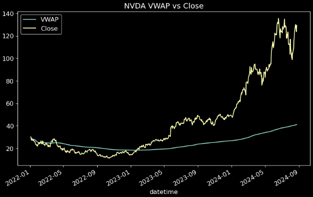
Inferences:
- A stock trading above the VWAP as the line rises indicates an uptrend and vice versa on a downtrend.
- VWAP is a simple line that acts as a support if the stock is trading above it (cf. 2023–2024) and a resistance if the stock is trading below it (cf. 2022).
NVDA Fundamental Analysis
- Fundamental and technical analysis are two common ways to sort and pick stocks [10].
- For example, a trader might use fundamental metrics to select the candidate and technical indicators to identify a specific entry or exit price.
- Let’s learn how to use financial statements to decide if NVDA is a good investment.
- Reading the company info
import yfinance as yf
nvda=yf.Ticker("NVDA")
print(nvda.info)

{'address1': '2788 San Tomas Expressway', 'city': 'Santa Clara', 'state': 'CA', 'zip': '95051', 'country': 'United States', 'phone': '408 486 2000', 'website': 'https://www.nvidia.com', 'industry': 'Semiconductors', 'industryKey': 'semiconductors', 'industryDisp': 'Semiconductors', 'sector': 'Technology',
..........

'revenueGrowth': 2.621, 'grossMargins': 0.75286, 'ebitdaMargins': 0.61768, 'operatingMargins': 0.64925003, 'financialCurrency': 'USD', 'trailingPegRatio': 1.4497}- Reading the nvda.info dictionary keys
nvda_info=nvda.info
nvda_info.keys()

dict_keys(['address1', 'city', 'state', 'zip', 'country', 'phone', 'website', 'industry', 'industryKey', 'industryDisp', 'sector', 'sectorKey', 'sectorDisp', 'longBusinessSummary', 'fullTimeEmployees', 'companyOfficers', 'auditRisk', 'boardRisk', 'compensationRisk', 'shareHolderRightsRisk', 'overallRisk', 'governanceEpochDate', 'compensationAsOfEpochDate', 'irWebsite', 'maxAge', 'priceHint', 'previousClose', 'open', 'dayLow', 'dayHigh', 'regularMarketPreviousClose', 'regularMarketOpen', 'regularMarketDayLow', 'regularMarketDayHigh', 'dividendRate', 'dividendYield', 'exDividendDate', 'payoutRatio', 'fiveYearAvgDividendYield', 'beta', 'trailingPE', 'forwardPE', 'volume', 'regularMarketVolume', 'averageVolume', 'averageVolume10days', 'averageDailyVolume10Day', 'bid', 'ask', 'bidSize', 'askSize', 'marketCap', 'fiftyTwoWeekLow', 'fiftyTwoWeekHigh', 'priceToSalesTrailing12Months', 'fiftyDayAverage', 'twoHundredDayAverage', 'trailingAnnualDividendRate', 'trailingAnnualDividendYield', 'currency', 'enterpriseValue', 'profitMargins', 'floatShares', 'sharesOutstanding', 'sharesShort', 'sharesShortPriorMonth', 'sharesShortPreviousMonthDate', 'dateShortInterest', 'sharesPercentSharesOut', 'heldPercentInsiders', 'heldPercentInstitutions', 'shortRatio', 'shortPercentOfFloat', 'impliedSharesOutstanding', 'bookValue', 'priceToBook', 'lastFiscalYearEnd', 'nextFiscalYearEnd', 'mostRecentQuarter', 'earningsQuarterlyGrowth', 'netIncomeToCommon', 'trailingEps', 'forwardEps', 'pegRatio', 'lastSplitFactor', 'lastSplitDate', 'enterpriseToRevenue', 'enterpriseToEbitda', '52WeekChange', 'SandP52WeekChange', 'lastDividendValue', 'lastDividendDate', 'exchange', 'quoteType', 'symbol', 'underlyingSymbol', 'shortName', 'longName', 'firstTradeDateEpochUtc', 'timeZoneFullName', 'timeZoneShortName', 'uuid', 'messageBoardId', 'gmtOffSetMilliseconds', 'currentPrice', 'targetHighPrice', 'targetLowPrice', 'targetMeanPrice', 'targetMedianPrice', 'recommendationMean', 'recommendationKey', 'numberOfAnalystOpinions', 'totalCash', 'totalCashPerShare', 'ebitda', 'totalDebt', 'quickRatio', 'currentRatio', 'totalRevenue', 'debtToEquity', 'revenuePerShare', 'returnOnAssets', 'returnOnEquity', 'freeCashflow', 'operatingCashflow', 'earningsGrowth', 'revenueGrowth', 'grossMargins', 'ebitdaMargins', 'operatingMargins', 'financialCurrency', 'trailingPegRatio'])- Examining the key fundamental KPIs
nvda_info['beta']
1.68

#As of today (2024-08-19), NVIDIA's Beta is 2.49.

nvda_info['trailingPegRatio']
1.4497

nvda_info['earningsGrowth']
6.5

nvda_info['totalRevenue']
79773999104

nvda_info['debtToEquity']
22.866

nvda_info['revenuePerShare']
3.234

nvda_info['ebitda']
49274998784

nvda_info['overallRisk']
8- Printing the NVDA financial statement
rio=yf.Ticker("NVDA")
rio.financials 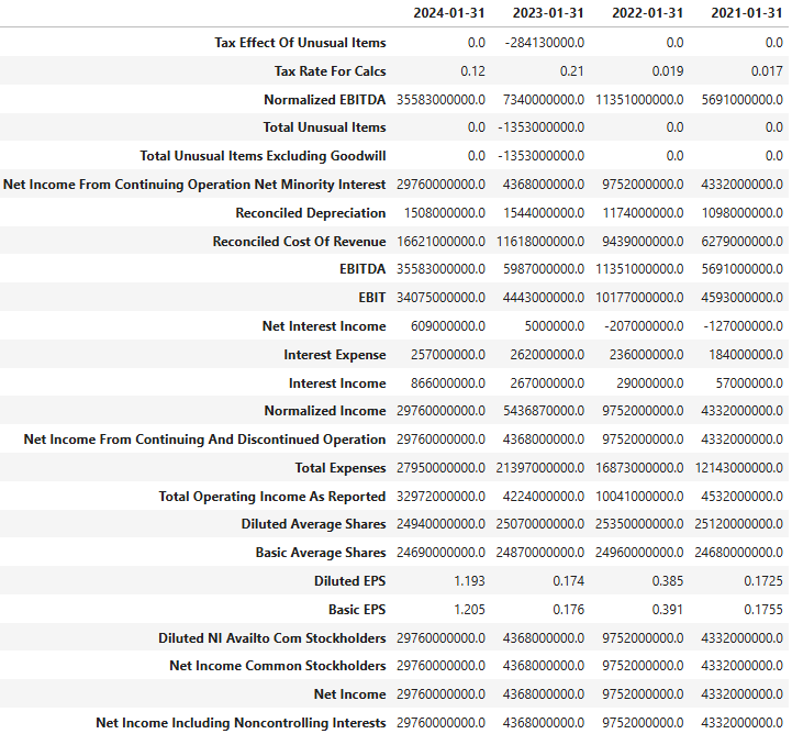
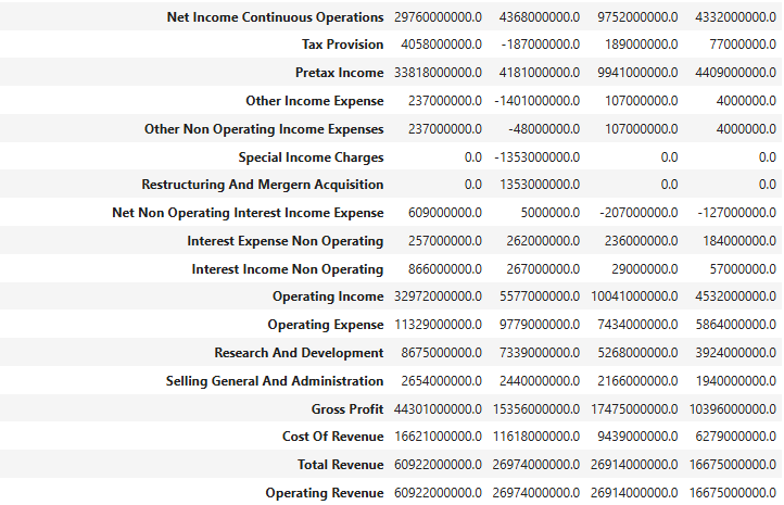
Inferences:
- The beta is 1.68, so NVIDIA’s price volatility has been higher than the market average.
- The Risk Score for NVIDIA Corp. is significantly higher than its peer group’s. This means that NVIDIA Corp. is significantly less risky than its peer group.
- Conventional wisdom says that a PEG ratio of 1 or less is considered good (at par or undervalued to its growth rate). A value greater than 1, in general, is not as good (overvalued to its growth rate).
- NVIDIA 2024 annual Diluted EPS was $1.19, a 585.63% increase from 2023.
- NVDA Debt/Equity (D/E) Ratio is ~0.2, whereas INTC D/E ~ 0.46 (April 28, 2024).
- NVDA Revenue Per Share (ttm) is 3.23.
Backtesting NVDA Williams %R & MACD Trading Strategy
- This section is about combining the Williams %R (WR) and MACD indicators to create a hybrid WR-MACD trading strategy that maximizes the expected returns by avoiding false trading signals [11–13].
- Williams %R is a momentum indicator that oscillates from 0 to -100. Readings from 0 to -20 are considered overbought. Readings from -80 to -100 are considered oversold. This indicator determines the market’s current level in relation to the lookback period’s highest high.
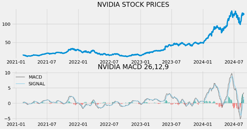
- The MACD indicator can help traders identify significant changes in momentum and market sentiment, providing insights for entering and exiting a trade. The lines on the histogram oscillate around the zero line and that gives the MACD the characteristic of the oscillator. The deeper or higher the lines, the stronger the move in price.
- When the MACD lines are above the zero horizontal, the market can be said to be bullish, and when they are below, we are in bearish mode.
- When the signal line crosses the MACD line, the indicator is said to be generating a potential buy (above signal line) or sell indication (below signal line).
- Reading the input stock data (being referred to as DAT2)
# IMPORTING PACKAGES

import numpy as np
import pandas as pd
import matplotlib.pyplot as plt
import requests
from math import floor
from termcolor import colored as cl

plt.style.use('fivethirtyeight')
plt.rcParams['figure.figsize'] = (12,6)

# EXTRACTING STOCK DATA

import pandas as pd
import numpy as np
import requests
import matplotlib.pyplot as plt
from math import floor
from termcolor import colored as cl

plt.style.use('fivethirtyeight')
plt.rcParams['figure.figsize'] = (12,6)

def get_historical_data(symbol, start_date):
    api_key = 'YOUR API KEY'
    api_url = f'https://api.twelvedata.com/time_series?symbol={symbol}&interval=1day&outputsize=5000&apikey={api_key}'
    raw_df = requests.get(api_url).json()
    df = pd.DataFrame(raw_df['values']).iloc[::-1].set_index('datetime').astype(float)
    df = df[df.index >= start_date]
    df.index = pd.to_datetime(df.index)
    return df

aapl = get_historical_data('NVDA', '2021-01-01')
aapl.tail()

           open      high      low    close  volume
datetime
2024-08-22 130.02000 130.75000 123.10 123.74 376189100.0
2024-08-23 125.86000 129.60001 125.22 129.37 323230300.0
2024-08-26 129.57001 131.25999 124.37 126.46 331964700.0
2024-08-27 125.05000 129.20000 123.88 128.30 301726100.0
2024-08-28 128.12000 128.33000 122.64 124.85 266495961.0- Calculating and plotting the Williams %R and MACD indicators [13]
# WILLIAMS %R CALCULATION

def get_wr(high, low, close, lookback):
    highh = high.rolling(lookback).max()
    lowl = low.rolling(lookback).min()
    wr = -100 * ((highh - close) / (highh - lowl))
    return wr

aapl['wr_14'] = get_wr(aapl['high'], aapl['low'], aapl['close'], 14)
aapl.tail()

# WILLIAMS %R PLOT

plot_data = aapl[aapl.index >= '2021-01-01']

ax1 = plt.subplot2grid((11,1), (0,0), rowspan = 5, colspan = 1)
ax2 = plt.subplot2grid((11,1), (6,0), rowspan = 5, colspan = 1)
ax1.plot(plot_data['close'], linewidth = 2)
ax1.set_title('NVIDIA CLOSING PRICE')
ax2.plot(plot_data['wr_14'], color = 'orange', linewidth = 2)
ax2.axhline(-20, linewidth = 1.5, linestyle = '--', color = 'grey')
ax2.axhline(-80, linewidth = 1.5, linestyle = '--', color = 'grey')
ax2.set_title('NVIDIA WILLIAMS %R 14')
plt.show()

# MACD CALCULATION

def get_macd(price, slow, fast, smooth):
    exp1 = price.ewm(span = fast, adjust = False).mean()
    exp2 = price.ewm(span = slow, adjust = False).mean()
    macd = pd.DataFrame(exp1 - exp2).rename(columns = {'close':'macd'})
    signal = pd.DataFrame(macd.ewm(span = smooth, adjust = False).mean()).rename(columns = {'macd':'signal'})
    hist = pd.DataFrame(macd['macd'] - signal['signal']).rename(columns = {0:'hist'})
    return macd, signal, hist

aapl['macd'] = get_macd(aapl['close'], 26, 12, 9)[0]
aapl['macd_signal'] = get_macd(aapl['close'], 26, 12, 9)[1]
aapl['macd_hist'] = get_macd(aapl['close'], 26, 12, 9)[2]
aapl = aapl.dropna()
aapl.tail()

# MACD PLOT

plot_data = aapl[aapl.index >= '2021-01-01']

def plot_macd(prices, macd, signal, hist):
    ax1 = plt.subplot2grid((11,1), (0,0), rowspan = 5, colspan = 1)
    ax2 = plt.subplot2grid((11,1), (6,0), rowspan = 5, colspan = 1)

    ax1.plot(prices)
    ax1.set_title('NVIDIA STOCK PRICES')
    ax2.plot(macd, color = 'grey', linewidth = 1.5, label = 'MACD')
    ax2.plot(signal, color = 'skyblue', linewidth = 1.5, label = 'SIGNAL')
    ax2.set_title('NVIDIA MACD 26,12,9')

    for i in range(len(prices)):
        if str(hist[i])[0] == '-':
            ax2.bar(prices.index[i], hist[i], color = '#ef5350')
        else:
            ax2.bar(prices.index[i], hist[i], color = '#26a69a')

    plt.legend(loc = 'upper left')

plot_macd(plot_data['close'], plot_data['macd'], plot_data['macd_signal'], plot_data['macd_hist'])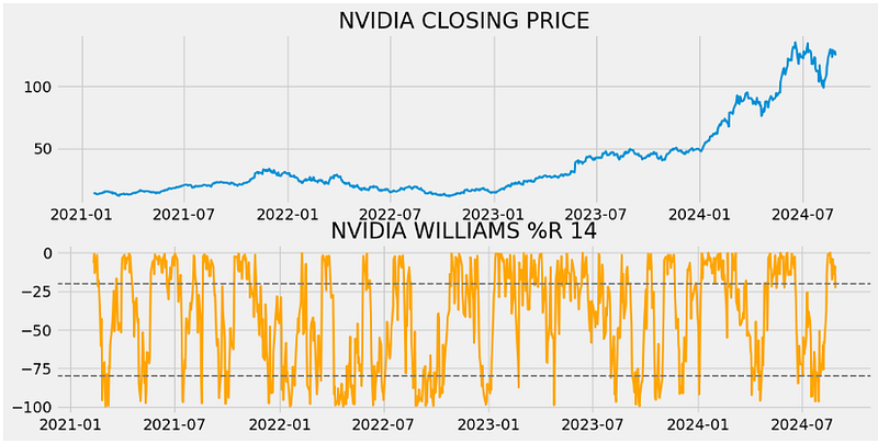
- Implementing the hybrid trading strategy and plotting the expected returns [13]
# TRADING STRATEGY

def implement_wr_macd_strategy(prices, wr, macd, macd_signal):
    buy_price = []
    sell_price = []
    wr_macd_signal = []
    signal = 0

    for i in range(len(wr)):
        if macd[i] > macd_signal[i]:
            if signal != 1:
                buy_price.append(prices[i])
                sell_price.append(np.nan)
                signal = 1
                wr_macd_signal.append(signal)
            else:
                buy_price.append(np.nan)
                sell_price.append(np.nan)
                wr_macd_signal.append(0)

        elif macd[i] < macd_signal[i]:
            if signal != -1:
                buy_price.append(np.nan)
                sell_price.append(prices[i])
                signal = -1
                wr_macd_signal.append(signal)
            else:
                buy_price.append(np.nan)
                sell_price.append(np.nan)
                wr_macd_signal.append(0)

        else:
            buy_price.append(np.nan)
            sell_price.append(np.nan)
            wr_macd_signal.append(0)

    return buy_price, sell_price, wr_macd_signal

buy_price, sell_price, wr_macd_signal = implement_wr_macd_strategy(aapl['close'], aapl['wr_14'], aapl['macd'], aapl['macd_signal'])

# POSITION

position = []
for i in range(len(wr_macd_signal)):
    if wr_macd_signal[i] > 1:
        position.append(0)
    else:
        position.append(1)

for i in range(len(aapl['close'])):
    if wr_macd_signal[i] == 1:
        position[i] = 1
    elif wr_macd_signal[i] == -1:
        position[i] = 0
    else:
        position[i] = position[i-1]

close_price = aapl['close']
wr = aapl['wr_14']
macd_line = aapl['macd']
signal_line = aapl['macd_signal']
wr_macd_signal = pd.DataFrame(wr_macd_signal).rename(columns = {0:'wr_macd_signal'}).set_index(aapl.index)
position = pd.DataFrame(position).rename(columns = {0:'wr_macd_position'}).set_index(aapl.index)

frames = [close_price, wr, macd_line, signal_line, wr_macd_signal, position]
strategy = pd.concat(frames, join = 'inner', axis = 1)

strategy.head()

rets = aapl.close.pct_change().dropna()
strat_rets = strategy.wr_macd_position[1:]*rets

plt.title('NVIDIA Daily Returns')
rets.plot(color = 'blue', alpha = 0.3, linewidth = 7)
strat_rets.plot(color = 'r', linewidth = 1)
plt.show()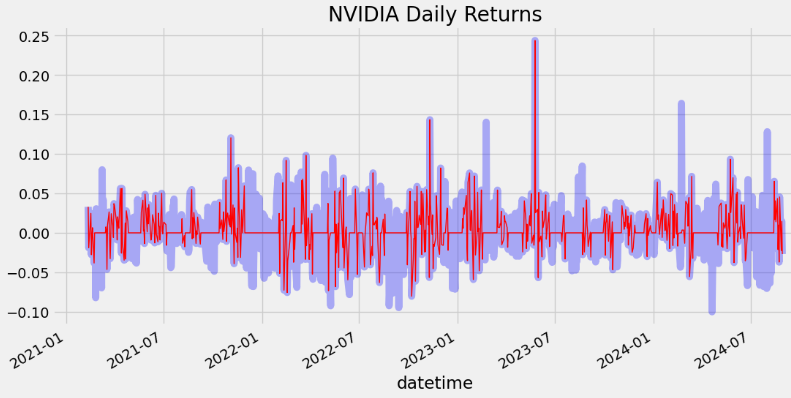
rets_cum = (1 + rets).cumprod() - 1
strat_cum = (1 + strat_rets).cumprod() - 1

plt.title('Cumulative Returns')
rets_cum.plot(color = 'blue', alpha = 0.3, linewidth = 7)
strat_cum.plot(color = 'r', linewidth = 2)
plt.show()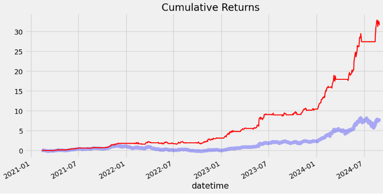
- Backtesting the hybrid strategy
aapl_ret = pd.DataFrame(np.diff(aapl['close'])).rename(columns = {0:'returns'})
adx_strategy_ret = []

for i in range(len(aapl_ret)):
    returns = aapl_ret['returns'][i]*strategy['wr_macd_position'][i]
    adx_strategy_ret.append(returns)

adx_strategy_ret_df = pd.DataFrame(adx_strategy_ret).rename(columns = {0:'returns'})
investment_value = 10000
number_of_stocks = floor(investment_value/aapl['close'][-1])
adx_investment_ret = []

for i in range(len(adx_strategy_ret_df['returns'])):
    returns = number_of_stocks*adx_strategy_ret_df['returns'][i]
    adx_investment_ret.append(returns)

adx_investment_ret_df = pd.DataFrame(adx_investment_ret).rename(columns = {0:'investment_returns'})
total_investment_ret = round(sum(adx_investment_ret_df['investment_returns']), 2)
profit_percentage = floor((total_investment_ret/investment_value)*100)
print(cl('Profit gained from the WR-MACD strategy by investing $10k in NVDA: {}'.format(total_investment_ret), attrs = ['bold']))
print(cl('Profit percentage of the WR-MACD strategy : {}%'.format(profit_percentage), attrs = ['bold']))

Profit gained from the WR-MACD strategy by investing $10k in NVDA: 6991.62
Profit percentage of the WR-MACD strategy : 69%- Comparing strategy profits to industry averages (SPY)
def get_benchmark(start_date, investment_value):
    spy = get_historical_data('SPY', start_date)['close']
    benchmark = pd.DataFrame(np.diff(spy)).rename(columns = {0:'benchmark_returns'})

    investment_value = investment_value
    number_of_stocks = floor(investment_value/spy[-1])
    benchmark_investment_ret = []

    for i in range(len(benchmark['benchmark_returns'])):
        returns = number_of_stocks*benchmark['benchmark_returns'][i]
        benchmark_investment_ret.append(returns)

    benchmark_investment_ret_df = pd.DataFrame(benchmark_investment_ret).rename(columns = {0:'investment_returns'})
    return benchmark_investment_ret_df

benchmark = get_benchmark('2021-01-01', 10000)

investment_value = 10000
total_benchmark_investment_ret = round(sum(benchmark['investment_returns']), 2)
benchmark_profit_percentage = floor((total_benchmark_investment_ret/investment_value)*100)
print(cl('Benchmark profit by investing $10k : {}'.format(total_benchmark_investment_ret), attrs = ['bold']))
print(cl('Benchmark Profit percentage : {}%'.format(benchmark_profit_percentage), attrs = ['bold']))
print(cl('WR-MACD Strategy profit is {}% higher than the Benchmark Profit'.format(profit_percentage - benchmark_profit_percentage), attrs = ['bold']))

Benchmark profit by investing $10k : 3178.83
Benchmark Profit percentage : 31%
WR-MACD Strategy profit is 38% higher than the Benchmark Profit
Inferences:
Profit gained from the WR-MACD strategy by investing $10k in NVDA: 6991.62
Profit percentage of the WR-MACD strategy : 69%
Benchmark profit by investing $10k : 3178.83
Benchmark Profit percentage : 31%
WR-MACD Strategy profit is 38% higher than the Benchmark Profit- Backtesting the WR-MACD strategy is important because it allows us to test this strategy on historical data (viz. DAT2) to evaluate its viability before risking capital in real-time trading.
- However, past data isn’t necessarily a good predictor of future market behavior, so no strategy can guarantee accuracy.
- Also, backtesting is different from scenario analysis and the forward performance approach to testing the effectiveness of a given trading strategy.
Monte Carlo Simulation of NVDA Value at Risk (VaR)
- In this section, we’ll download the NVDA historical data and calculate Value at Risk (VaR) by running the Monte Carlo simulation [14, 15].
- VaR quantifies the potential loss in value of an asset over a defined period for a given confidence interval [15].
- Importing Python libraries and downloading the NVDA stock data
import numpy
import pandas
import scipy.stats
import matplotlib.pyplot as plt
import requests
from math import floor
from termcolor import colored as cl
import numpy as np
import pandas as pd
plt.style.use("bmh")
from datetime import datetime

def get_historical_data(symbol, start_date):
    api_key = 'YOUR API KEY'
    api_url = f'https://api.twelvedata.com/time_series?symbol={symbol}&interval=1day&outputsize=5000&apikey={api_key}'
    raw_df = requests.get(api_url).json()
    df = pd.DataFrame(raw_df['values']).iloc[::-1].set_index('datetime').astype(float)
    df = df[df.index >= start_date]
    df.index = pd.to_datetime(df.index)
    return df

nvd = get_historical_data('NVDA', '2022-01-03')
nvd.tail()

           open      high      low    close   volume
datetime
2024-08-23 125.86000 129.60001 125.22 129.370 323230300.0
2024-08-26 129.57001 131.25999 124.37 126.460 331964700.0
2024-08-27 125.05000 129.20000 123.88 128.300 303134600.0
2024-08-28 128.12000 128.33000 122.64 125.610 437643900.0
2024-08-29 121.35500 124.11000 119.23 121.255 245155865.0- Plotting the NVDA close price
fig = plt.figure()
fig.set_size_inches(10,3)
nvd["close"].plot()
plt.title("NVDA stock", weight="bold");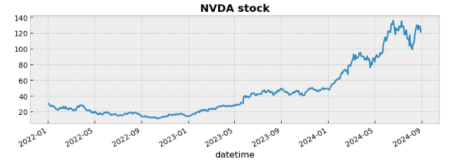
- Calculating the NVDA daily returns
fig = plt.figure()
fig.set_size_inches(10,3)
nvd["close"].pct_change().plot()
plt.title("NVDA daily returns", weight="bold");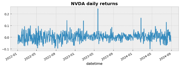
- Plotting the histogram of NVDA daily returns and calculating std
nvd["close"].pct_change().hist(bins=50, density=True, histtype="stepfilled", alpha=0.5)
plt.title("Histogram of NVDA daily returns", weight="bold")
nvd["close"].pct_change().std()

0.03567997781131377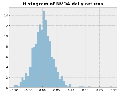
- Calculating the normal probability Q-Q plot of NVDA daily returns
Q = nvd["close"].pct_change().dropna()
scipy.stats.probplot(Q, dist=scipy.stats.norm, plot=plt.figure().add_subplot(111))
plt.title("Normal probability plot of NVDA daily returns", weight="bold");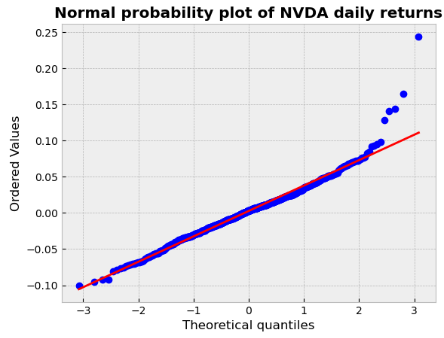
- Calculating the student probability Q-Q plot of NVDA daily returns
tdf, tmean, tsigma = scipy.stats.t.fit(Q)
scipy.stats.probplot(Q, dist=scipy.stats.t, sparams=(tdf, tmean, tsigma), plot=plt.figure().add_subplot(111))
plt.title("Student probability plot of NVDA daily returns", weight="bold");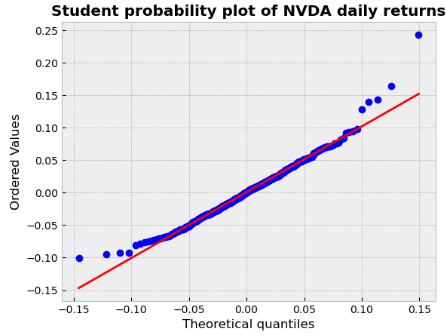
- Calculating empirical quantiles from a histogram of daily returns
returns = nvd["close"].pct_change().dropna()
mean = returns.mean()
sigma = returns.std()
tdf, tmean, tsigma = scipy.stats.t.fit(returns)
returns.hist(bins=40, density=True, histtype="stepfilled", alpha=0.5)
plt.title("NVDA Daily Returns", weight="bold");


returns.quantile(0.05)

-0.05528745219087147

print (mean,sigma)

0.0027153437382872237 0.03567997781131377

scipy.stats.norm.ppf(0.05, mean, sigma)

-0.055972997174200304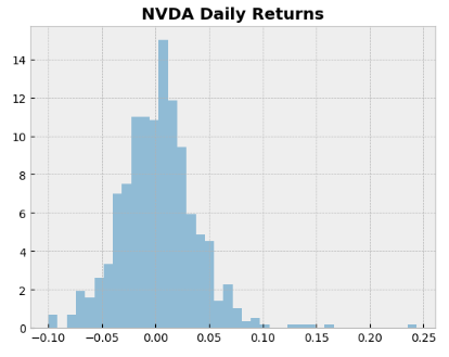
- Plotting the PDF approximation of the above empirical distribution
support = numpy.linspace(returns.min(), returns.max(), 100)
returns.hist(bins=40, density=True, histtype="stepfilled", alpha=0.5);
plt.plot(support, scipy.stats.t.pdf(support, loc=tmean, scale=tsigma, df=tdf), "r-")
plt.title("Daily change in NVDA (%)", weight="bold");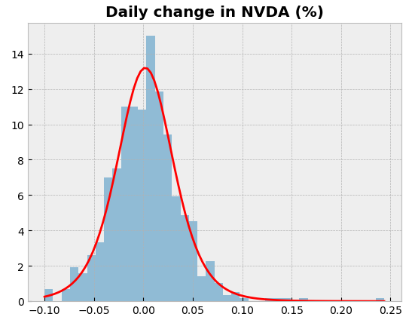
- Running the following Monte Carlo simulation using the function random_walk. This function simulates one stock market evolution, and returns the price evolution as an array. It simulates geometric Brownian motion using pseudorandom numbers drawn from a normal distribution [14].
days = 300 # time horizon
dt = 1/float(days)
sigma = 0.03567997781131377 # volatility
mu = 0.0027153437382872237 # drift (average growth rate)
startprice=121.255
def random_walk(startprice):
price = numpy.zeros(days)
shock = numpy.zeros(days)
price[0] = startprice
for i in range(1, days):
shock[i] = numpy.random.normal(loc=mu * dt, scale=sigma * numpy.sqrt(dt))
price[i] = max(0, price[i-1] + shock[i] * price[i-1])
return price
plt.figure(figsize=(9,4))
for run in range(300):
plt.plot(random_walk(startprice))
plt.xlabel("Days")
plt.ylabel("Price USD");
runs = 10000
simulations = numpy.zeros(runs)
for run in range(runs):
simulations[run] = random_walk(startprice)[days-1]
q = numpy.percentile(simulations, 1)
plt.hist(simulations, density=True, bins=30, histtype="stepfilled", alpha=0.5)
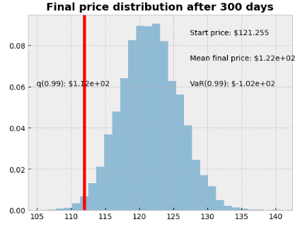
plt.figtext(0.6, 0.8, "Start price: $121.255")
plt.figtext(0.6, 0.7, "Mean final price: ${:.3}".format(simulations.mean()))
plt.figtext(0.6, 0.6, "VaR(0.99): ${:.3}".format(10 - q))
plt.figtext(0.15, 0.6, "q(0.99): ${:.3}".format(q))
plt.axvline(x=q, linewidth=4, color="r")
plt.title("Final price distribution after {} days".format(days), weight="bold");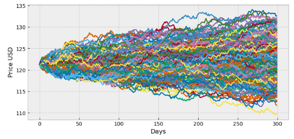
Inferences:
- Student’s t distribution seems to fit better than the normal distribution (cf. the r.h.s. tail of the distribution).
- The 0.05 empirical quantile of daily returns is at -0.055. That means that with 95% confidence, our worst daily loss will not exceed 5.5%. If we have a $1 M investment, our one-day 5% VaR is 0.055 * $1 M = $55 k.
- Final price is spread out between $110 (our portfolio has lost value) to almost $134. We can see that the expectation (mean outcome) is a profit; this is due to the fact that the drift in our random walk (parameter mu) is positive.
- Our big Monte Carlo simulation of random walks yields the probability distribution of the final price and quantile measures for the estimated VaR.
- We have looked at the 1% empirical quantile of the final price distribution to estimate the VaR, which is $102 for a $121.255 investment.
Read more here.
NVDA RSI & Bollinger Bands Support-Resistance
- RSI with Bollinger Bands is a technical indicator combining two popular tools in the world of trading and investing: the Relative Strength Index (RSI) and Bollinger Bands (BB) [17, 18].
- Reading the NVDA historical stock data DAT3
import pandas as pd
import matplotlib.pyplot as plt
import numpy as np
import requests
from termcolor import colored as cl
from math import floor
# Import seaborn
import seaborn as sns

plt.style.use('fivethirtyeight')
plt.rcParams['figure.figsize'] = (12,6)

# EXTRACTING STOCK DATA

def get_historical_data(symbol, start_date):
    api_key = 'a07d718849d64be78e8a7d5669e4e3af'
    api_url = f'https://api.twelvedata.com/time_series?symbol={symbol}&interval=1day&outputsize=5000&apikey={api_key}'
    raw_df = requests.get(api_url).json()
    df = pd.DataFrame(raw_df['values']).iloc[::-1].set_index('datetime').astype(float)
    df = df[df.index >= start_date]
    df.index = pd.to_datetime(df.index)
    return df

ticker='NVDA'
start='2023-01-01'

stock = get_historical_data(ticker, start)
stock.tail()

           open      high      low     close volume
datetime
2024-08-23 125.86000 129.60001 125.22 129.37 323230300.0
2024-08-26 129.57001 131.25999 124.37 126.46 331964700.0
2024-08-27 125.05000 129.20000 123.88 128.30 303134600.0
2024-08-28 128.12000 128.33000 122.64 125.61 448101100.0
2024-08-29 121.36000 124.43000 116.71 117.59 451799100.0

stock['Date']=stock.index- Calculating the RSI and Bollinger Bands indicators [17]
#Calculate relative strength of stock in time period (days)
def calculate_relative_strength(data, time_period):

    #set date as index
    data = data.set_index(data['Date'])

    #create delta
    delta = data['close'].diff(1)

    #create gains and loss variables
    up = delta.copy()
    down = delta.copy()

    #conditional to set delta gain
    up[up < 0] = 0
    down[down > 0] = 0

    #get average of gains
    AVG_gain = up.rolling(window = time_period).mean()

    #get average of loss
    AVG_loss = abs(down.rolling(window = time_period).mean())
    return (AVG_gain, AVG_loss)

#Calculates RSI
def calculate_RSI(AVG_gain, AVG_loss):

    # Calculate relative strength
    RS = AVG_gain/AVG_loss

    #Calculate relative strength index
    RSI = 100.0-(100.0/(1.0+RS))
    return RSI

#Plot RSI
def plot_RSI(RSI, tick_symbol):

    #set plot sizes
    plt.figure(figsize=(18,8))

    #plot RSI values against date index
    plot = sns.lineplot(x = RSI.index, y = RSI.values)
    plot.set_title("RSI: " + tick_symbol)
    plot.set_ylabel('Relative Strength Index')

    #plot all levels in RSI
    plot.axhline(30, color = 'green')
    plot.axhline(70, color = 'green')
    plot.axhline(20, color = 'yellow')
    plot.axhline(80, color = 'yellow')
    plot.axhline(10, color = 'red')
    plot.axhline(90, color = 'red')

    #Get the last/current RSI
    data = RSI.tail(1)

    #If greater than 70, display "Sell"
    if data.values > 70:
        for x,y in zip(data.index,data.values):
            label = "Sell"
            plt.annotate(label, # this is the text
                         (x,y), # this is the point to label
                         textcoords="offset points", # how to position the text
                         xytext=(0,10), # distance from text to points (x,y)
                         ha='center',
                         fontsize = 25) # horizontal alignment can be left, right or center
            plt.scatter(data.index, data.values,label = 'Sell', marker = 'v', color = 'red', alpha = 1, s = 100) #plot scatter on RSI plot
    #If less than 30, display "Buy"
    elif data.values < 30:
        for x,y in zip(data.index,data.values):
            label = "Buy"
            plt.annotate(label, # this is the text
                         (x,y), # this is the point to label
                         textcoords="offset points", # how to position the text
                         xytext=(0,10), # distance from text to points (x,y)
                         ha='center',
                         fontsize = 25) # horizontal alignment can be left, right or center
            plt.scatter(data.index, data.values, label = 'Buy', marker = '^', color = 'green', alpha = 1, s = 100) #plot scatter on RSI plot

#Combine all smaller elements to single function
def RSI(data, tick_symbol, time_period):
        gain, loss = calculate_relative_strength(data, time_period)
        RSI = calculate_RSI(gain, loss)
        plot_RSI(RSI, tick_symbol)

# Produces the bollinger bands for a stock
def Bollinger_Band(data, period, ticker):
        plt.figure(figsize=(18,8))
        data['bollinger_first'] = data['close'].rolling(period).mean()
        #Use formula
        data['bollinger_second'] = data['close'].rolling(period).mean() + 2*(data['close'].rolling(period).std())
        data['bollinger_third'] = data['close'].rolling(period).mean() - 2*(data['close'].rolling(period).std())

        #signal to determine upper and lower band crossovers
        buy = []
        sell = []
        for i in range(len(data['close'])):
            if data['close'][i] > data['bollinger_second'][i]:
                buy.append(np.nan)
                sell.append(data['close'][i])
            elif data['close'][i] < data['bollinger_third'][i]:
                buy.append(data['close'][i])
                sell.append(np.nan)
            else:
                buy.append(np.nan)
                sell.append(np.nan)

        #plot result
        graph = sns.lineplot(data = data, x = 'Date', y = 'close')
        sns.lineplot(data = data, x = 'Date', y = 'bollinger_second')
        sns.lineplot(data = data, x = 'Date', y = 'bollinger_first')
        sns.lineplot(data = data, x = 'Date', y = 'bollinger_third')
#        plt.legend(['Close Price', 'Upper Band', 'Middle Band', 'Lower Bound'])
        graph.set_title("Bollinger Bands:" + ticker)

        #create columns for buy and sell signals
        data['Buy'] = buy
        data['Sell'] = sell

        #obtain non-null records
        data_buy_non_nan = data.loc[data['Buy'].notnull()]
        data_sell_non_nan = data.loc[data['Sell'].notnull()]

        #concatenate signals
        signals = pd.concat([data_buy_non_nan, data_sell_non_nan])
        signals = signals.reset_index(drop = True)

        #plot signals

        sns.scatterplot(data=data, x="Date", y="Buy",s=400, c="green", marker="^")
        sns.scatterplot(data=data, x="Date", y="Sell",s=400, c="red", marker="v")

        #Add close price on signals
        for x,y,z in zip(signals['Date'], signals['close'], signals['close']):
            label = z #Label corresponds to labels in dataset
            plt.annotate(label, #text to be displayed
                         (x,y), #point for the specific label
                         textcoords="offset points", #positioning of the text
                         xytext=(0,10), #distance from text to points
                         ha='center',
                         fontsize = 12) #horizontal alignment


#Combine all RSI and Bollinger Band functions into one
def RSI_Bollinger(data, period_bollinger, period_RSI, ticker):
    fig = plt.figure()
    bollinger = Bollinger_Band(data, period_bollinger, ticker)
    rsi = RSI(data, ticker, period_RSI)
    bollinger
    rsi
plt.show()- Applying RSI with Bollinger Bands to DAT3 and visualize the result
if __name__ == "__main__":
#    period_RSI = int(input('Time period of RSI (in days)'))
    period_RSI = 14
    #specify period for bollinger 20
#    period_Boll = int(input('Time period of Bollinger Band (in days)'))
    period_Boll=20
    #view results
    RSI_Bollinger(stock, period_Boll, period_RSI, ticker)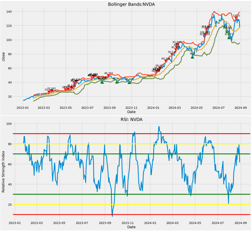
- RSI is considered overbought when above 70 and oversold when below 30.
- The Bollinger Bands widen and narrow when the volatility of the price is higher or lower, respectively.
- When the price bounces off of the upper band and crosses the middle band, then the lower band becomes the price target.
Inferences:
- The current NVDA RSI value is below 70 and well above 30, suggesting NVDA is neither overbought nor oversold (i.e. Oversold / Overbought: Neutral / Hold).
- 20 Day Bollinger Bands also suggest Hold.
- Widening Bands indicate an increase in price volatility, which often signals the start of a strong trend (as of 2024–08–29).
Risk-Return Comparison of 10 Stocks to Watch
- Let’s implement the passive investment strategy [19] by computing risks and returns of the following 10 stocks to watch:
symbol =['AMD','GOOGL','WST','DXCM','NVDA','AAPL','AMZN','NFLX','TSLA','MSFT']- Fetching and plotting the stock historical data DAT4
import numpy as np
import pandas as pd
from datetime import date
import matplotlib.pyplot as plt
import yfinance as yf
%matplotlib inline

start_date = '2020-01-01'

df = yf.download(symbol, start=start_date)['Close'] #getting only Closing price values
df.tail()

Ticker AAPL AMD AMZN DXCM GOOGL MSFT NFLX NVDA TSLA WST
Date
2024-08-26 227.179993 149.990005 175.500000 73.669998 166.160004 413.489990 688.440002 126.459999 213.210007 303.489990
2024-08-27 228.029999 150.500000 173.119995 72.239998 164.679993 413.839996 695.719971 128.300003 209.210007 302.630005
2024-08-28 226.490005 146.360001 170.800003 70.480003 162.850006 410.600006 683.840027 125.610001 205.750000 297.609985
2024-08-29 229.789993 145.490005 172.119995 69.620003 161.779999 413.119995 692.479980 117.589996 206.279999 314.790009
2024-08-30 228.794998 146.804993 173.960007 69.389801 161.919998 414.600006 691.049988 118.459999 208.804993 317.730011

#Charting the stock prices for multiple stocks
fig = plt.figure(figsize=(20,12))
ax1 = fig.add_subplot(4,3,1)
ax2 = fig.add_subplot(4,3,2)
ax3 = fig.add_subplot(4,3,3)
ax4 = fig.add_subplot(4,3,4)
ax5 = fig.add_subplot(4,3,5)
ax6 = fig.add_subplot(4,3,6)
ax7 = fig.add_subplot(4,3,7)
ax8 = fig.add_subplot(4,3,8)
ax9 = fig.add_subplot(4,3,9)
ax10 = fig.add_subplot(4,3,10)
ax1.plot(df['AMZN'])
ax1.set_title("Amazon")
ax2.plot(df['AMD'])
ax2.set_title("AMD")
ax3.plot(df['GOOGL'])
ax3.set_title("Google")
ax4.plot(df['NFLX'])
ax4.set_title("Netflix")
ax5.plot(df['WST'])
ax5.set_title("WST")
ax6.plot(df['DXCM'])
ax6.set_title("DXCM")
ax7.plot(df['NVDA'])
ax7.set_title("NVDA")
ax8.plot(df['TSLA'])
ax8.set_title("Tesla")
ax9.plot(df['AAPL'])
ax9.set_title("AAPL")
ax10.plot(df['MSFT'])
ax10.set_title("MSFT")
plt.tight_layout()
plt.show()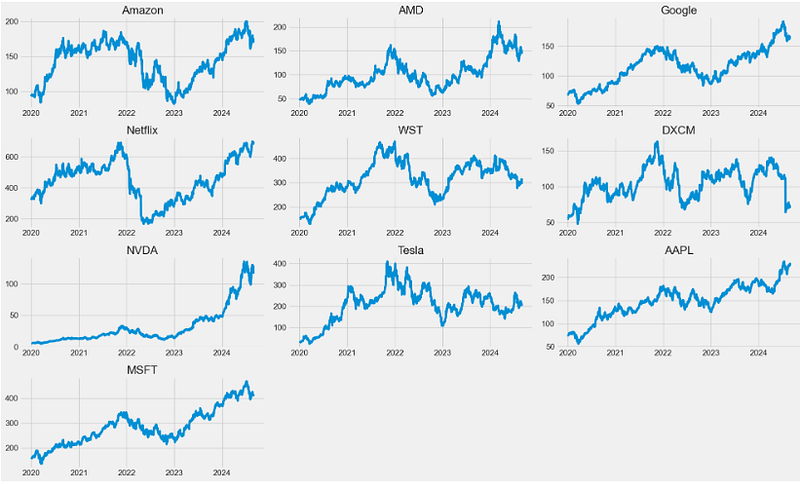
- Calculating portfolio return of the hold strategy
log_returns_stock=np.exp(log_returns.sum())#total return of hold strategy
log_returns_stock

Ticker
AAPL      3.047045
AMD       2.989918
AMZN      1.833078
DXCM      1.265198
GOOGL     2.366075
MSFT      2.581248
NFLX      2.095297
NVDA     19.750740
TSLA      7.279494
WST       2.093911
dtype: float64

portfolio_return=log_returns_stock.mean(axis=0)
print("Portfolio return using hold strategy: {:>10.2%}".format(portfolio_return))

Portfolio return using hold strategy:    453.02%

fig, ax= plt.subplots(figsize=(12,8))
for c in log_returns:
    ax.plot(log_returns.index, 100*(np.exp(log_returns[c].cumsum()) - 1), label=str(c))
ax.set_ylabel('Total relative returns (%)')
ax.set_xlabel('Time period')
ax.set_title('Portfolio return using hold strategy')
ax.legend(loc='best')
plt.show()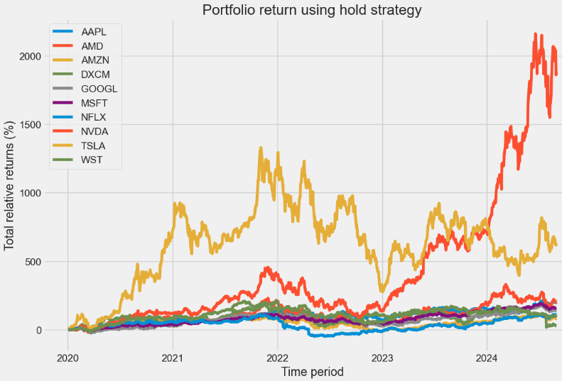
- Comparing asset risks and returns of the hold strategy
returns = log_returns #using log_return
plt.figure(figsize=(12,6))
plt.scatter(returns.mean(), returns.std(),s=100)
plt.xlabel('Expected returns')
plt.ylabel('Risk')
for label, x, y in zip(returns.columns, returns.mean(), returns.std()):
    plt.annotate(
        label,
        xy = (x, y), xytext = (50, 30),
        textcoords = 'offset points', ha = 'right', va = 'bottom',
        arrowprops=dict(arrowstyle= '<|-|>',
                             color='blue',
                             lw=1,
                             ls='--'))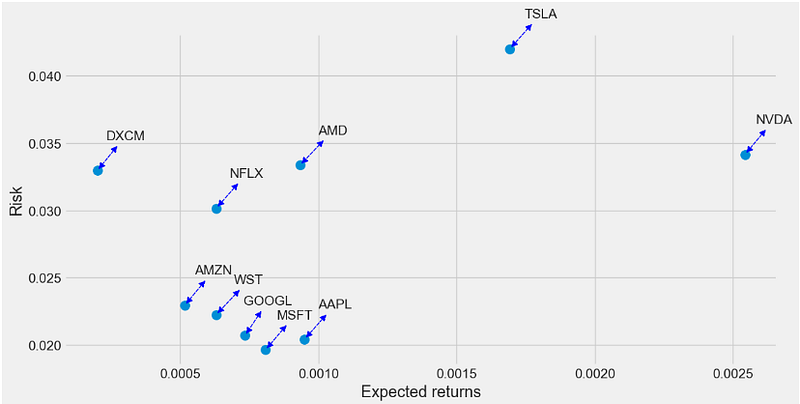
- Calculating returns of the SMA 50–200 trading strategy [19]
# Calculating the short-window moving average for entire portfolio
short_rolling= df.rolling(window=50,min_periods=1).mean()
df_short = short_rolling.add_suffix('_short')
# Calculating the long-window moving average for entire portfolio
long_rolling = df.rolling(window=200,min_periods=1).mean()
df_long = long_rolling.add_suffix('_long')
#to join two tables into one df
new_df=pd.concat([df_short,df_long],axis=1)
#calculating trading for entire portfolio
new_df['AMD_Trade'] = np.where(new_df['AMD_short']> new_df['AMD_long'], 1, -1)
new_df['AMZN_Trade'] = np.where(new_df['AMZN_short']> new_df['AMZN_long'], 1, -1)
new_df['AAPL_Trade'] = np.where(new_df['AAPL_short']> new_df['AAPL_long'], 1, -1)
new_df['DXCM_Trade'] = np.where(new_df['DXCM_short']> new_df['DXCM_long'], 1, -1)
new_df['MSFT_Trade'] = np.where(new_df['MSFT_short']> new_df['MSFT_long'], 1, -1)
new_df['NFLX_Trade'] = np.where(new_df['NFLX_short']> new_df['NFLX_long'], 1, -1)
new_df['NVDA_Trade'] = np.where(new_df['NVDA_short']> new_df['NVDA_long'], 1, -1)
new_df['TSLA_Trade'] = np.where(new_df['TSLA_short']> new_df['TSLA_long'], 1, -1)
new_df['WST_Trade'] = np.where(new_df['WST_short']> new_df['WST_long'], 1, -1)
new_df['GOOGL_Trade'] = np.where(new_df['GOOGL_short']> new_df['GOOGL_long'], 1, -1)
# creating return column
log_returns = np.log(df).diff()
df_return= log_returns.add_suffix('_Return')
new_df=pd.concat([df_return,new_df],axis=1)
#remove NA values
new_df.dropna(inplace=True)
#calculating instatenious rate of return
new_df['AMD_Treturn']=new_df.AMD_Return*new_df.AMD_Trade
AMD_total_treturn=np.exp(new_df.AMD_Treturn.sum())
print('AMD_total_treturn is:',AMD_total_treturn)
new_df['AMZN_Treturn']=new_df.AMZN_Return*new_df.AMZN_Trade
AMZN_total_treturn=np.exp(new_df.AMZN_Treturn.sum())
print('AMZN_total_treturn is:',AMZN_total_treturn)
new_df['AAPL_Treturn']=new_df.AAPL_Return*new_df.AAPL_Trade
AAPL_total_treturn=np.exp(new_df.AAPL_Treturn.sum())
print('AAPL_total_treturn is:',AAPL_total_treturn)
new_df['DXCM_Treturn']=new_df.DXCM_Return*new_df.DXCM_Trade
DXCM_total_treturn=np.exp(new_df.DXCM_Treturn.sum())
print('DXCM_total_treturn is:',DXCM_total_treturn)
new_df['MSFT_Treturn']=new_df.MSFT_Return*new_df.MSFT_Trade
MSFT_total_treturn=np.exp(new_df.MSFT_Treturn.sum())
print('MSFT_total_treturn is:',MSFT_total_treturn)
new_df['NFLX_Treturn']=new_df.NFLX_Return*new_df.NFLX_Trade
NFLX_total_treturn=np.exp(new_df.NFLX_Treturn.sum())
print('NFLX_total_treturn is:',NFLX_total_treturn)
new_df['NVDA_Treturn']=new_df.NVDA_Return*new_df.NVDA_Trade
NVDA_total_treturn=np.exp(new_df.NVDA_Treturn.sum())
print('NVDA_total_treturn is:',NVDA_total_treturn)
new_df['TSLA_Treturn']=new_df.TSLA_Return*new_df.TSLA_Trade
TSLA_total_treturn=np.exp(new_df.TSLA_Treturn.sum())
print('TSLA_total_treturn is:',TSLA_total_treturn)
new_df['WST_Treturn']=new_df.WST_Return*new_df.WST_Trade
WST_total_treturn=np.exp(new_df.WST_Treturn.sum())
print('WST_total_treturn is:',WST_total_treturn)
new_df['GOOGL_Treturn']=new_df.GOOGL_Return*new_df.GOOGL_Trade
GOOGL_total_treturn=np.exp(new_df.GOOGL_Treturn.sum())
print('GOOGL_total_treturn is;',GOOGL_total_treturn)

AMD_total_treturn is: 2.3799707255030196
AMZN_total_treturn is: 3.1633346327179472
AAPL_total_treturn is: 0.8448978146082059
DXCM_total_treturn is: 1.1943644380013865
MSFT_total_treturn is: 2.4911794060806116
NFLX_total_treturn is: 4.234814819819454
NVDA_total_treturn is: 26.215899221614798
TSLA_total_treturn is: 1.7373723016290843
WST_total_treturn is: 1.8016621963389188
GOOGL_total_treturn is; 2.6805537913562865

treturns_total = [AMD_total_treturn,AMZN_total_treturn,AAPL_total_treturn,DXCM_total_treturn,MSFT_total_treturn,NFLX_total_treturn,NVDA_total_treturn,TSLA_total_treturn,WST_total_treturn,GOOGL_total_treturn]
potrfolio_trade_strategy = sum(treturns_total) / len(treturns_total)
print("Portfolio return using trade strategy: {:>10.2%}".format(potrfolio_trade_strategy))

Portfolio return using trade strategy:    467.44%
Inferences:
- We have implemented moving average based strategies to buy and/or sell stocks for 10 stocks of interest and compared the results with the ones obtained when using the buy and hold strategy.
- We can see that the SMA 50–200 trading strategy performed better than the buy and hold strategy with 467% and 453% returns, respectively.
- The Risk-Return plot shows that NVDA has max expected return and medium risk; DXCM has min expected return and medium risk; MSFT has medium expected return and min risk; TSLA has high expected return (second after NVDA) and max risk.
- This is a part of debate that has been going on for decades. Buy and Hold vs. Timing the Market: Which one is better?
Backtest GOOG RSI-SMA Trading Strategies
- Let’s backtest GOOG RSI-SMA trading strategies by installing Backtesting 0.3.3
!pip install backtesting
- Reading the GOOG stock data and backtesting the RSI-SMA trading strategies [20]
import pandas as pd

def SMA(array, n):
    """Simple moving average"""
    return pd.Series(array).rolling(n).mean()

def RSI(array, n):
    """Relative strength index"""
    # Approximate; good enough
    gain = pd.Series(array).diff()
    loss = gain.copy()
    gain[gain < 0] = 0
    loss[loss > 0] = 0
    rs = gain.ewm(n).mean() / loss.abs().ewm(n).mean()
    return 100 - 100 / (1 + rs)

import backtesting

from backtesting import Strategy, Backtest
from backtesting.lib import resample_apply


class System(Strategy):
    d_rsi = 30  # Daily RSI lookback periods
    w_rsi = 30  # Weekly
    level = 70

    def init(self):
        # Compute moving averages the strategy demands
        self.ma10 = self.I(SMA, self.data.Close, 10)
        self.ma20 = self.I(SMA, self.data.Close, 20)
        self.ma50 = self.I(SMA, self.data.Close, 50)
        self.ma100 = self.I(SMA, self.data.Close, 100)

        # Compute daily RSI(30)
        self.daily_rsi = self.I(RSI, self.data.Close, self.d_rsi)

        # To construct weekly RSI, we can use `resample_apply()`
        # helper function from the library
        self.weekly_rsi = resample_apply(
            'W-FRI', RSI, self.data.Close, self.w_rsi)


    def next(self):
        price = self.data.Close[-1]

        # If we don't already have a position, and
        # if all conditions are satisfied, enter long.
        if (not self.position and
            self.daily_rsi[-1] > self.level and
            self.weekly_rsi[-1] > self.level and
            self.weekly_rsi[-1] > self.daily_rsi[-1] and
            self.ma10[-1] > self.ma20[-1] > self.ma50[-1] > self.ma100[-1] and
            price > self.ma10[-1]):

            # Buy at market price on next open, but do
            # set 8% fixed stop loss.
            self.buy(sl=.92 * price)

        # If the price closes 2% or more below 10-day MA
        # close the position, if any.
        elif price < .98 * self.ma10[-1]:
            self.position.close()

import yfinance as yf
GOOGLE=yf.download("GOOG",start="2020-01-01", auto_adjust = True)

from backtesting import Backtest

backtest = Backtest(GOOGLE, System, commission=.002)
stats= backtest.run()

%%time

backtest.optimize(d_rsi=range(10, 35, 5),
                  w_rsi=range(10, 35, 5),
                  level=range(30, 80, 10))

Error displaying widget
CPU times: total: 4.45 s
Wall time: 4.48 s
Start                     2020-01-02 00:00:00
End                       2024-08-30 00:00:00
Duration                   1702 days 00:00:00
Exposure Time [%]                   35.860307
Equity Final [$]                 18418.236525
Equity Peak [$]                  19330.237563
Return [%]                          84.182365
Buy & Hold Return [%]              141.774928
Return (Ann.) [%]                   14.008097
Volatility (Ann.) [%]               17.698778
Sharpe Ratio                         0.791473
Sortino Ratio                        1.422444
Calmar Ratio                         1.178269
Max. Drawdown [%]                   -11.88871
Avg. Drawdown [%]                   -3.297176
Max. Drawdown Duration      617 days 00:00:00
Avg. Drawdown Duration       48 days 00:00:00
# Trades                                   14
Win Rate [%]                             50.0
Best Trade [%]                      16.859706
Worst Trade [%]                     -6.881568
Avg. Trade [%]                       4.478954
Max. Trade Duration         116 days 00:00:00
Avg. Trade Duration          43 days 00:00:00
Profit Factor                        5.857247
Expectancy [%]                       4.737138
SQN                                  2.272172
_strategy                 System(d_rsi=10,...
_equity_curve                             ...
_trades                       Size  EntryB...
dtype: object

backtest.plot()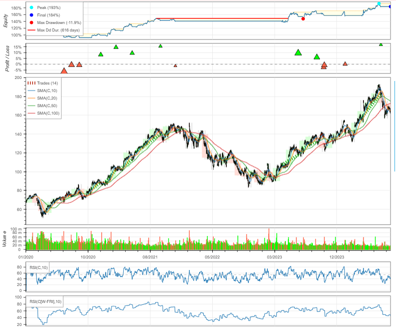
Inferences:
- This example shows some of the features of backtesting.py, a Python framework for backtesting trading strategies.
Backtest.run() method returns a pandas Series of simulation results and statistics associated with our strategy.
Backtest.plot() method provides the same insights in a more visual form.
- We see that this simple strategy makes almost 84% return in the period of 2020–2024, with annual volatility 18%, max drawdown 12%, and with max drawdown period spanning 617 days.
Sortino Ratio 1.422444- A good Sortino ratio typically exceeds 1. It measures the risk-adjusted returns, focusing on downside risk. A higher Sortino ratio indicates better performance in managing downside volatility, which is crucial for risk-averse investors.
Calmar Ratio 1.178269- If the Calamar ratio is more than 1, it indicates that the returns are higher than the drawdown, albeit slightly.
Sharpe Ratio 0.791473- Investments with less than 1.00 Sharpe Ratio do not generate high returns. Contrarily, investments with a Sharpe Ratio of 1.00 to 3.00 or above have higher returns subsequently.
AMD SMA-MACD-ADX Trend-Following Analysis
- Let’s evaluate statistical trends in the recent AMD trading activity, involving technical indicators such as SMA, MACD [21], and ADX [22]. The idea is to combine these three indicators for a comprehensive trend-following trading strategy.
- The Simple Moving Average (SMA) indicator smooths price data to reveal the underlying trend. The 200-day SMA is particularly useful for long-term analysis, indicating the overall trend direction.
- MACD [21], short for moving average convergence/divergence, can help traders identify significant changes in momentum and market sentiment. When the MACD line crosses from below to above the signal line, the indicator is considered bullish. The further below the zero line the stronger the signal. When the MACD line crosses from above to below the signal line, the indicator is considered bearish.
- Traders use the MACD histogram to identify potential trend reversals and price swings. If MACD is below its signal line, the histogram will be below the MACD’s baseline. Zeroes in the MACD histogram occur when the MACD line crosses higher than the signal line (generally considered a buy signal) or below the signal line (a sell signal). Peaks and troughs in the histogram indicate when a burst of bearish or bullish momentum is losing strength, and the curve is likely to return to its mean.
- The ADX value typically ranges from 0 to 100. ADX Value vs Trend Strength: 0–25 Absent or Weak Trend; 25–50 Strong Trend; 50–75 Very Strong Trend; 75–100 Extremely Strong Trend.
- Reading the AMD stock data DAT5 and examining the general data info
import yfinance as yf
ticker = 'AMD'
start_date = dt.datetime(2020,1,1)

df = yf.download(ticker, start=start_date, interval="1d")
df.tail()

           Open       High       Low        Close      Adj Close  Volume
Date
2024-08-26 154.699997 158.279999 148.910004 149.990005 149.990005 49893300
2024-08-27 150.130005 151.699997 148.440002 150.500000 150.500000 35102700
2024-08-28 149.399994 150.429993 144.720001 146.360001 146.360001 34075800
2024-08-29 146.589996 149.490005 144.470001 145.490005 145.490005 31602100
2024-08-30 147.520004 148.990005 145.250000 148.559998 148.559998 31139700

df.shape
(1174, 6)

df.info()
<class 'pandas.core.frame.DataFrame'>
DatetimeIndex: 1174 entries, 2020-01-02 to 2024-08-30
Data columns (total 6 columns):
 #   Column     Non-Null Count  Dtype
---  ------     --------------  -----
 0   Open       1174 non-null   float64
 1   High       1174 non-null   float64
 2   Low        1174 non-null   float64
 3   Close      1174 non-null   float64
 4   Adj Close  1174 non-null   float64
 5   Volume     1174 non-null   int64
dtypes: float64(5), int64(1)
memory usage: 64.2 KB

df['Close'].describe().T
count    1174.000000
mean      100.648152
std        35.210767
min        38.709999
25%        78.097498
50%        93.584999
75%       118.262499
max       211.380005
Name: Close, dtype: float64- Plotting the AMD candlesticks
import mplfinance as mpf
import matplotlib.pyplot as plt

# Plot candlestick chart
mpf.plot(df, type="candle", style="yahoo", title="AMD Stock Price 2020-2024")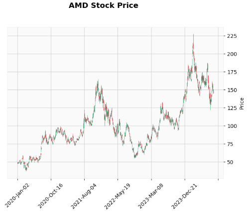
- Examining the AMD daily and cumulative returns
amd_daily_returns = df['Adj Close'].pct_change()
amd_daily_returns.plot(title='AMD Daily Returns')
plt.grid()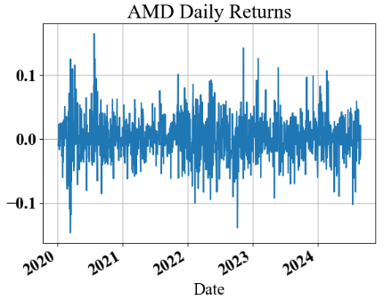
amd_daily_returns.hist()

amd_daily_returns.std()
0.0334299238200219

amd_daily_returns.kurt()
2.102226488552409

amd_daily_returns.skew()
0.18632525165901895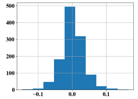
amd_cum_returns=amd_daily_returns.add(1).cumprod().sub(1)
amd_cum_returns.plot(title='AMD Cumulative Returns')
plt.grid()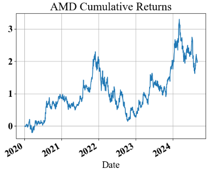
- Implementing the SMA50–200 crossover strategy [22]
dff = df.copy()
# Calculate 50-day and 200-day moving averages
dff['SMA50'] = dff['Close'].rolling(window=50).mean()
dff['SMA200'] = dff['Close'].rolling(window=200).mean()

# Generate trading signals based on moving average crossover
dff['Signal'] = 0
dff['Signal'][50:] = dff['SMA50'][50:] > dff['SMA200'][50:]
dff['Position'] = dff['Signal'].diff()

plt.figure(figsize=(12, 8))
plt.plot(dff['Close'], label='USD Close Price')
plt.plot(dff['SMA50'], label='50-day SMA')
plt.plot(dff['SMA200'], label='200-day SMA')
plt.plot(dff[dff['Position'] == 1].index, dff['SMA50'][dff['Position'] == 1], '^', markersize=20, color='g', label='Buy signal')
plt.plot(dff[dff['Position'] == -1].index, dff['SMA50'][dff['Position'] == -1], 'v', markersize=20, color='r', label='Sell signal')
plt.title('AMD Simple Moving Average Crossover Strategy')
plt.xlabel('Date')
plt.ylabel('Price')
plt.legend()
plt.show()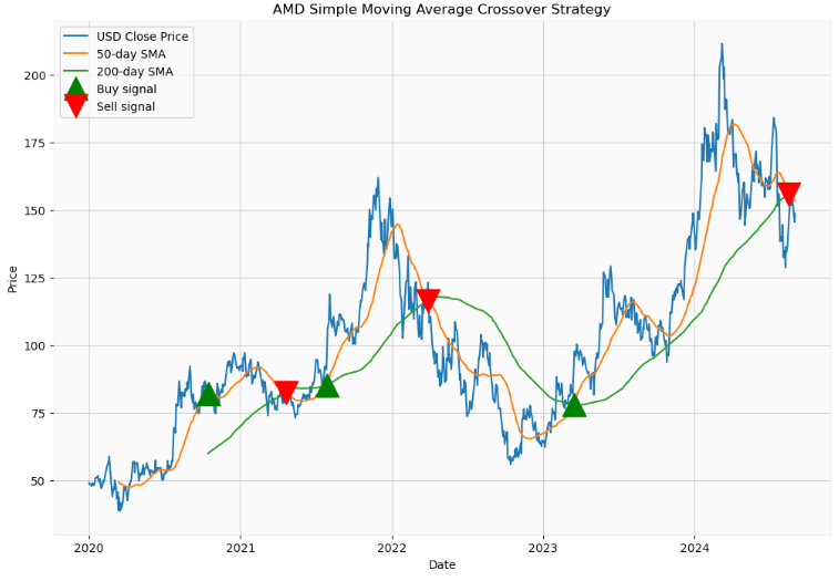
- Calculating the AMD MACD (12–26–9) trading indicator [21, 22]
def MACD(ohlc, period_fast = 12, period_slow = 26,signal = 9,column = "Close",adjust = True):
        """
        MACD, MACD Signal and MACD difference.
        The MACD Line oscillates above and below the zero line, which is also known as the centerline.
        These crossovers signal that the 12-day EMA has crossed the 26-day EMA. The direction, of course, depends on the direction of the moving average cross.
        Positive MACD indicates that the 12-day EMA is above the 26-day EMA. Positive values increase as the shorter EMA diverges further from the longer EMA.
        This means upside momentum is increasing. Negative MACD values indicates that the 12-day EMA is below the 26-day EMA.
        Negative values increase as the shorter EMA diverges further below the longer EMA. This means downside momentum is increasing.

        Signal line crossovers are the most common MACD signals. The signal line is a 9-day EMA of the MACD Line.
        As a moving average of the indicator, it trails the MACD and makes it easier to spot MACD turns.
        A bullish crossover occurs when the MACD turns up and crosses above the signal line.
        A bearish crossover occurs when the MACD turns down and crosses below the signal line.
        """

        EMA_fast = pd.Series(
            ohlc[column].ewm(ignore_na=False, span=period_fast, adjust=adjust).mean(),
            name="EMA_fast",
        )
        EMA_slow = pd.Series(
            ohlc[column].ewm(ignore_na=False, span=period_slow, adjust=adjust).mean(),
            name="EMA_slow",
        )
        MACD = pd.Series(EMA_fast - EMA_slow, name="MACD")
        MACD_signal = pd.Series(
            MACD.ewm(ignore_na=False, span=signal, adjust=adjust).mean(), name="SIGNAL"
        )

        return pd.concat([MACD, MACD_signal], axis=1)

plt.figure(figsize=(14,6))
dff[["MACD", "MACD_signal"]]=MACD(dff, period_fast = 12, period_slow = 26,signal = 9,column = "Close",adjust = True)
dff['MACD'].plot(label='MACD')
dff['MACD_signal'].plot(label='MACD_signal')
#plt.ylabel('Price USD')
plt.title('AMD MACD (12-26-9)')
plt.legend()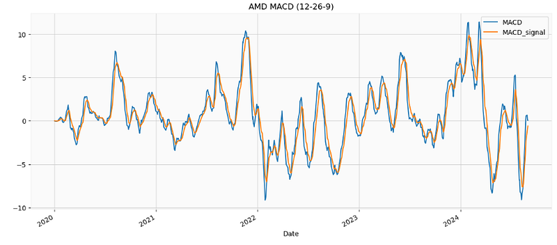
- Plotting the AMD MACD Histogram (12–26–9) [21]
# Calculate MACD
short_term = 12
long_term = 26
signal_period = 9

# Calculate short-term and long-term EMAs
short_ema = dff['Close'].ewm(span=short_term, adjust=False).mean()
long_ema = dff['Close'].ewm(span=long_term, adjust=False).mean()

# Calculate MACD Line
macd_line = short_ema - long_ema

# Calculate Signal Line
signal_line = macd_line.ewm(span=signal_period, adjust=False).mean()

# Calculate MACD Histogram
macd_histogram = macd_line - signal_line

# Add MACD components to the DataFrame
dff['MACD12269'] = macd_line
dff['Signal12269'] = signal_line
dff['Histogram12269'] = macd_histogram

import plotly.graph_objects as go

# Create a Plotly figure
fig = go.Figure()

# MACD and Signal lines
#fig.add_trace(go.Scatter(x=dff.index, y=dff['MACD12269'], mode='lines', name='MACD'))
#fig.add_trace(go.Scatter(x=dff.index, y=dff['Signal12269'], mode='lines', name='Signal'))

# Histogram
fig.add_trace(go.Bar(x=dff.index, y=dff['Histogram12269'], name='Histogram',
                marker_color=['green' if val >= 0 else 'red' for val in dff['Histogram12269']]))

# Customize the chart
fig.update_xaxes(rangeslider=dict(visible=False))
fig.update_layout(plot_bgcolor='#efefff', font_family='Monospace', font_color='#000000', font_size=20,width=400)
fig.update_layout(
        title="AMD MACD Histogram (12-26-9)"
 )

fig.update_layout(
    autosize=False,
    width=1100,
    height=500,
    margin=dict(
        l=50,
        r=50,
        b=100,
        t=100,
        pad=4
    ),
    paper_bgcolor="LightSteelBlue",
)

fig.update_layout(
     xaxis=dict(showgrid=True,gridwidth=1, gridcolor='Grey'),
     yaxis=dict(showgrid=True,gridwidth=1, gridcolor='Grey')
)
# Show the chart
fig.show()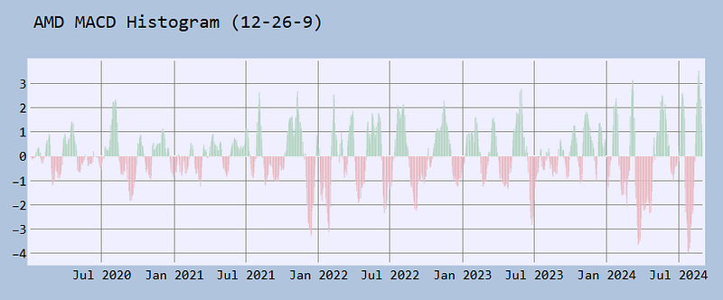
- Computing and plotting the AMD ADX20 indicator
def TR(ohlc,high="High",low="Low",close="Close"):
        """True Range is the maximum of three price ranges.
        Most recent period's high minus the most recent period's low.
        Absolute value of the most recent period's high minus the previous close.
        Absolute value of the most recent period's low minus the previous close."""

        TR1 = pd.Series(ohlc[high] - ohlc[low]).abs()  # True Range = High less Low

        TR2 = pd.Series(
            ohlc[high] - ohlc[close].shift()
        ).abs()  # True Range = High less Previous Close

        TR3 = pd.Series(
            ohlc[close].shift() - ohlc[low]
        ).abs()  # True Range = Previous Close less Low

        _TR = pd.concat([TR1, TR2, TR3], axis=1)

        _TR["TR"] = _TR.max(axis=1)

        return pd.Series(_TR["TR"], name="TR")

def ATR(ohlc, period = 14,high="High",low="Low",close="Close"):
        """Average True Range is moving average of True Range."""

        mytr=TR(ohlc,high=high,low=low,close=close)
        return pd.Series(
            mytr.rolling(center=False, window=period).mean(),
            name="{0} period ATR".format(period),
        )

def DMI(ohlc, period = 14, adjust = True,high="High",low="Low",close="Close"):
        """The directional movement indicator (also known as the directional movement index - DMI) is a valuable tool
         for assessing price direction and strength. This indicator was created in 1978 by J. Welles Wilder, who also created the popular
         relative strength index. DMI tells you when to be long or short.
         It is especially useful for trend trading strategies because it differentiates between strong and weak trends,
         allowing the trader to enter only the strongest trends.
        source: https://www.tradingview.com/wiki/Directional_Movement_(DMI)#CALCULATION

        :period: Specifies the number of Periods used for DMI calculation
        """

        ohlc["up_move"] = ohlc[high].diff()
        ohlc["down_move"] = -ohlc[low].diff()

        # positive Dmi
        def _dmp(row):
            if row["up_move"] > row["down_move"] and row["up_move"] > 0:
                return row["up_move"]
            else:
                return 0

        # negative Dmi
        def _dmn(row):
            if row["down_move"] > row["up_move"] and row["down_move"] > 0:
                return row["down_move"]
            else:
                return 0

        ohlc["plus"] = ohlc.apply(_dmp, axis=1)
        ohlc["minus"] = ohlc.apply(_dmn, axis=1)

        diplus = pd.Series(
            100
            * (ohlc["plus"] / ATR(ohlc, period = period,high=high,low=low,close=close))
            .ewm(alpha=1 / period, adjust=adjust)
            .mean(),
            name="DI+",
        )
        diminus = pd.Series(
            100
            * (ohlc["minus"] / ATR(ohlc, period = period,high=high,low=low,close=close))
            .ewm(alpha=1 / period, adjust=adjust)
            .mean(),
            name="DI-",
        )

        return pd.concat([diplus, diminus], axis=1)

def ADX(ohlc, period = 14, adjust = True,high="High",low="Low",column="Close"):
        """The A.D.X. is 100 * smoothed moving average of absolute value (DMI +/-) divided by (DMI+ + DMI-). ADX does not indicate trend direction or momentum,
        only trend strength. Generally, A.D.X. readings below 20 indicate trend weakness,
        and readings above 40 indicate trend strength. An extremely strong trend is indicated by readings above 50"""

        dmi = DMI(ohlc, period = period, adjust = adjust,high=high,low=low,close=column)
        return pd.Series(
            100
            * (abs(dmi["DI+"] - dmi["DI-"]) / (dmi["DI+"] + dmi["DI-"]))
            .ewm(alpha=1 / period, adjust=adjust)
            .mean(),
            name="{0} period ADX.".format(period),
        )

plt.figure(figsize=(12,6))
dff["ADX"]=ADX(dff, period = 20, adjust = True,high="High",low="Low",column="Close")
dff['ADX'].plot(label='ADX20')
plt.title('AMD ADX')
plt.legend()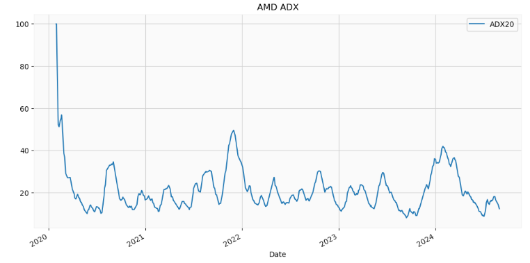
Inferences:
- The AMD’s total return over the DAT5 period is 200%.
- STD of daily returns is 3.3%.
- The kurtosis and histogram of daily returns indicate that the corresponding empirical distribution is close to normal distribution (kurtosis=3.0) with short tails.
- The positive skewness<0.5 of daily returns shows that the right-skewed distribution is almost symmetrical. The positive skewness of a distribution indicates that an investor may expect frequent small losses and a few large gains from the investment.
- The AMD SMA50–200 crossover strategy generates a sell signal or “death cross” at the end of the DAT5 period when a 50-day moving average crosses below a 200-day moving average.
- A zero line crossover: Since the MACD crosses below the zero line, the market is bearish and a short sell signal. However, positive MACD histogram bars indicate increasing upward momentum.
- The 20.00 ADX level acts as a tiebreaker: if the ADX is below the 20.00 level, price is in a range or in a very weak trend and only when the ADX breaks above the 20.00 level, it signals a strong trend that is likely to continue.
Conclusions
- This paper has addressed the intersection of Algorithmic Trading and Technical Analysis of top growth stocks.
- While technical analysis aims to decipher market trends and patterns, algorithmic trading utilizes the speed and precision of computer algorithms to optimize trade execution.
- Specific results of the present study can be summarized as follows:
The Sharpe Ratio of Top 7 Tech Stocks
- AMZN, GOOG, META, and MSFT have SR<1.0. A ratio under 1.0 is considered sub-optimal.
- AAPL and TSLA have the SR values of 0.97 and 1.04, respectively. A SR of close to 1.0 or greater is typically considered good.
- NVDA has the SR of 1.63 that is higher than the other 6 tech stocks.
- In risk-adjusted terms, NVDA would be the most acceptable investment opportunity.
NVDA PSR & 95% CI
- Combinations of skewness and kurtosis in returns distribution impact the STD and the confidence bands of the SR.
- The PSR metric accounts for the STD and uncertainty associated with estimating SR (Type I errors) [5].
NVDA Daily/Cumulative Returns
- Cumulative returns are the total gains or losses of an investment over a specific period. It is a crucial metric that investors use to determine the overall performance of their portfolio.
- This information can help investors adjust their portfolio to maximize their returns.
- However, taxes can substantially reduce the cumulative returns for most investments unless they are held in tax-advantaged accounts.
NVDA Keltner Channel (KC) Strategy
- We can see that the KC delivers powerful breakouts signals. The incorporation of ATR ensures that the KC is more effective when volatility rises [6].
- Traders can join a bullish breakout early when there is a pullback to the outside of the upper line. Likewise, when a bearish breakout occurs, traders can seek to place aggressive sell orders when the price pulls back to the outside of the lower line [6].
- The expected ROI of the KC trading strategy by investing $100k in NVDA is 123%.
- Results show that the KC trading strategy has outperformed the SPY ETF by 109%.
NVDA VWAP Support & Resistance
- A stock trading above the VWAP as the line rises indicates an uptrend and vice versa on a downtrend.
- VWAP is a simple line that acts as a support if the stock is trading above it (cf. 2023–2024) and a resistance if the stock is trading below it (cf. 2022).
NVDA Fundamental Analysis
- The beta is 1.68, so NVIDIA’s price volatility has been higher than the market average.
- The Risk Score for NVIDIA Corp. is significantly higher than its peer group’s. This means that NVIDIA Corp. is significantly less risky than its peer group.
- Conventional wisdom says that a PEG ratio of 1 or less is considered good (at par or undervalued to its growth rate). A value greater than 1, in general, is not as good (overvalued to its growth rate).
- NVIDIA 2024 annual Diluted EPS was $1.19, a 585.63% increase from 2023.
- NVDA Debt/Equity (D/E) Ratio is ~0.2, whereas INTC D/E ~ 0.46 (April 28, 2024).
- NVDA Revenue Per Share (ttm) is 3.23.
Backtesting NVDA Williams %R & MACD Trading Strategy
- Backtesting the WR-MACD strategy is important because it allows us to test this strategy on historical data (viz. DAT2) to evaluate its viability before risking capital in real-time trading.
- However, past data isn’t necessarily a good predictor of future market behavior, so no strategy can guarantee accuracy.
- Also, backtesting is different from scenario analysis and the forward performance approach to testing the effectiveness of a given trading strategy.
Monte Carlo Simulation of NVDA Value-at-Risk (VaR)
- Student’s t distribution seems to fit better than the normal distribution (cf. the r.h.s. tail of the distribution).
- The 0.05 empirical quantile of daily returns is at -0.055. That means that with 95% confidence, our worst daily loss will not exceed 5.5%. If we have a $1 M investment, our one-day 5% VaR is 0.055 * $1 M = $55 k.
- Final price is spread out between $110 (our portfolio has lost value) to almost $134. We can see that the expectation (mean outcome) is a profit; this is due to the fact that the drift in our random walk (parameter mu) is positive.
- Our big Monte Carlo simulation of random walks yields the probability distribution of the final price and quantile measures for the estimated VaR.
- We have looked at the 1% empirical quantile of the final price distribution to estimate the VaR, which is $102 for a $121.255 investment.
NVDA RSI & Bollinger Bands Support-Resistance
- The current NVDA RSI value is below 70 and well above 30, suggesting NVDA is neither overbought nor oversold (i.e. Oversold / Overbought: Neutral / Hold).
- 20 Day Bollinger Bands also suggest Hold.
- Widening Bands indicate an increase in price volatility, which often signals the start of a strong trend (as of 2024–08–29).
Risk-Return Comparison of 10 Stocks to Watch
- We have implemented moving average based strategies to buy and/or sell stocks for 10 stocks of interest and compared the results with the ones obtained when using the buy and hold strategy.
- We can see that the SMA 50–200 trading strategy performed better than the buy and hold strategy with 467% and 453% returns, respectively.
- The Risk-Return plot shows that NVDA has max expected return and medium risk; DXCM has min expected return and medium risk; MSFT has medium expected return and min risk; TSLA has high expected return (second after NVDA) and max risk.
- This is a part of debate that has been going on for decades. Buy and Hold vs. Timing the Market: Which one is better?
Backtest GOOG RSI-SMA Trading Strategies
- This example shows some of the features of backtesting.py, a Python framework for backtesting trading strategies.
Backtest.run() method returns a pandas Series of simulation results and statistics associated with our strategy.
Backtest.plot() method provides the same insights in a more visual form.
- We see that this simple strategy makes almost 84% return in the period of 2020–2024, with annual volatility 18%, max drawdown 12%, and with max drawdown period spanning 617 days.
Sortino Ratio 1.422444- A good Sortino ratio typically exceeds 1. It measures the risk-adjusted returns, focusing on downside risk. A higher Sortino ratio indicates better performance in managing downside volatility, which is crucial for risk-averse investors.
Calmar Ratio 1.178269- If the Calamar ratio is more than 1, it indicates that the returns are higher than the drawdown, albeit slightly.
Sharpe Ratio 0.791473- Investments with less than 1.00 Sharpe Ratio do not generate high returns. Contrarily, investments with a Sharpe Ratio of 1.00 to 3.00 or above have higher returns subsequently.
AMD SMA-MACD-ADX Trend-Following Analysis:
- The AMD’s total return over the DAT5 period is 200%.
- STD of daily returns is 3.3%.
- The kurtosis and histogram of daily returns indicate that the corresponding empirical distribution is close to normal distribution (kurtosis=3.0) with short tails.
- The positive skewness<0.5 of daily returns shows that the right-skewed distribution is almost symmetrical. The positive skewness of a distribution indicates that an investor may expect frequent small losses and a few large gains from the investment.
- The AMD SMA50–200 crossover strategy generates a sell signal or “death cross” at the end of the DAT5 period when a 50-day moving average crosses below a 200-day moving average.
- A zero line crossover: Since the MACD crosses below the zero line, the market is bearish and a short sell signal. However, positive MACD histogram bars indicate increasing upward momentum.
- The 20.00 ADX level acts as a tiebreaker: if the ADX is below the 20.00 level, price is in a range or in a very weak trend and only when the ADX breaks above the 20.00 level, it signals a strong trend that is likely to continue.
Bottom Line:
We have looked at the key trends, case examples and best industry practices that set to accelerate the algo trading market growth in 2024 and beyond. Factors such as the increasing adoption of real-time data analytics, interactive visualizations, and the rising demand for automated trading systems substantiate the rapid algo trading industry growth in 3 key regions such as North America, Europe, and Asia.
References
- Risk and Returns: The Sharpe Ratio
- The Sharpe Ratio Defined
- Algorithmic Trading with the Keltner Channel in Python
- rubenbriones/Probabilistic-Sharpe-Ratio/<~tree/master/src>
- Is Your Sharpe Ratio Lying to You? Meet the Probabilistic Sharpe Ratio
- Mechanics and Calculation of Keltner Channel
- Keltner Channel
- Building a VWAP Indicator in Python
- I Tested a VWAP Strategy on the 50 Largest S&P 500 Companies. Here Are the Results
- How to Pick Stocks: Fundamentals vs. Technicals
- Increasing Stock Returns by Combining Williams %R and MACD in Python
- Algorithmic Trading with Williams %R in Python
- Algorithmic-Trading-with-Python/Advanced Strategies/ Williams%R_MACD.py
- Stock market trends and Value at Risk
- Value at Risk (VaR) and Its Implementation in Python
- Monte Carlo simulation using Black-Scholes for stock price in Python
- Algorithmic Trading with Python: The RSI-Bollinger Band Strategy
- Bollinger Band and RSI Strategy: An In-depth Analysis
- Buy And Hold Vs SMA Crossover: Big Profits With Simple Strategy
- SharmaVidhiHaresh/Backtesting-Trading-Strategies-with-Python
- MACD Analysis Made Easy with Python
- NVDA Technical Analysis using 75 Simplified FinTA Indicators
Relevant 3rd Party SaaS

Read more: Macroaxis AI Investment Opportunity

Read more: Track All Markets with TradingView

See the use-case example: OXY Stock Analysis, Thursday, 23 June 2022
Explore More
- DigHiSci Posts
- Portfolio Optimization (PO) of 25 Largest US Tech Stocks: A Four-Fold Risk/Return Analysis
- NVDA Technical Analysis using 75 Simplified FinTA Indicators
- Striking a Balance between Portfolio Returns & Sharpe Ratio with Three-Step SMA Scenario Testing
- Backtesting AMD Algo-Trading SMA Cross Strategy: Long/Short Auto Tuning vs Buy&Hold
- 2Y Big Techs Portfolio Diversification, Risk-Return Tradeoff and LSTM Price Prediction: AAPL, NVDA, META & AMZN
- How to Swing Algo-Trade Tech Stocks using the Qullamaggie’s Breakouts — 1. NVIDIA
- Backtesting Hybrid CI & MACD Trading Strategies for NVIDIA
- A Deeper Look at NVIDIA KST Algo-Trading Signals & Backtesting
- Algo-Trading NVIDIA with ADX & RSI Indicators
- An Algo-Trading Sneak Peek at Top AI-Powered Growth Stocks — 1. NVIDIA
Infographic
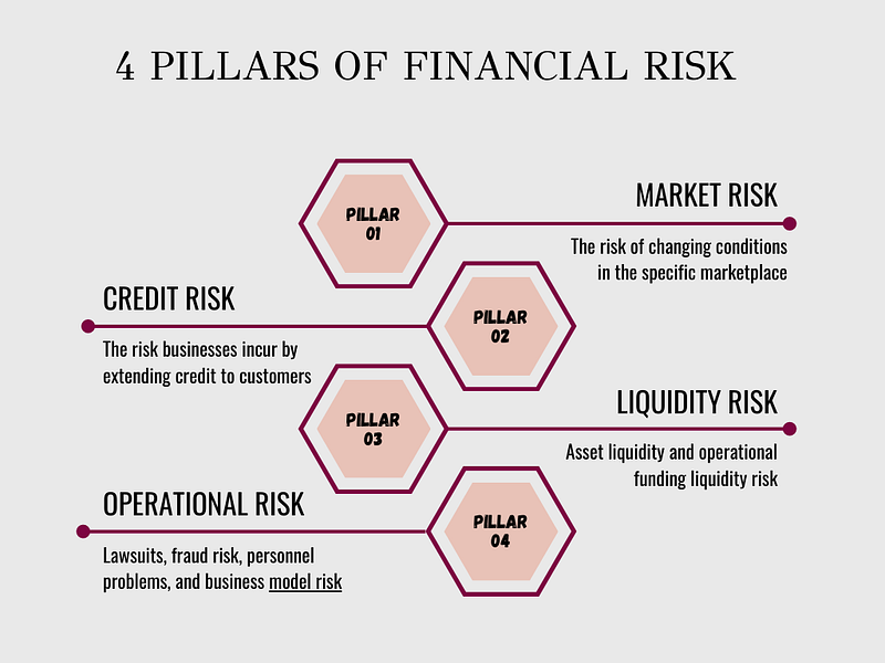
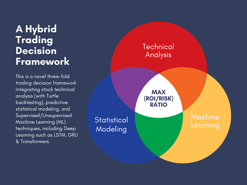
Read more:
- Leveraging Predictive Uncertainties of Time Series Forecasting Models
- A Market-Neutral Strategy
- Sales Forecasting: tslearn, Random Walk, Holt-Winters, SARIMAX, GARCH, Prophet, and LSTM
- Multiple-Criteria Technical Analysis of Blue Chips in Python
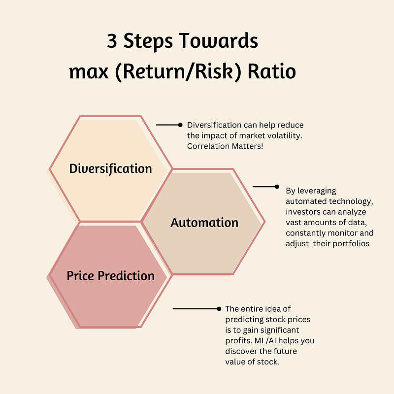

NVIDIA Rolling Volatility: GARCH & XGBoost
NVIDIA Returns-Drawdowns MVA & RNN Mean Reversal Trading


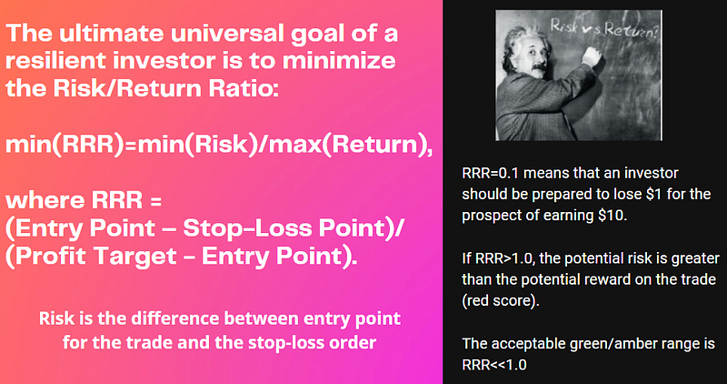
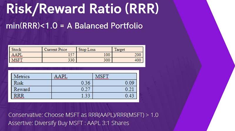
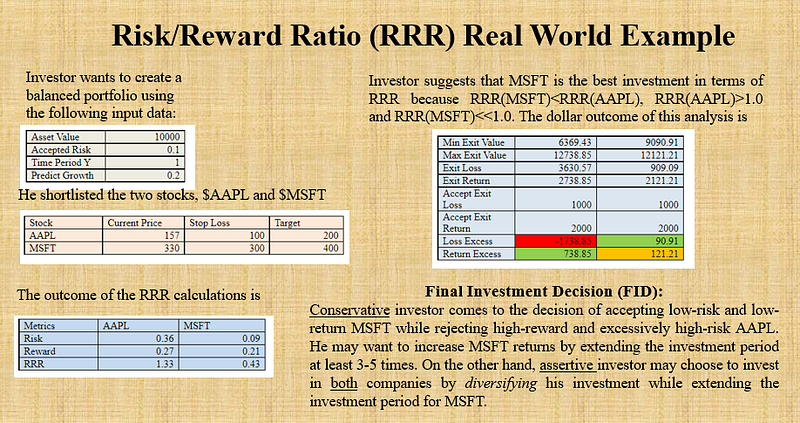

Read more: Invest in AI via Macroaxis Sep ’22 Update
Contacts
Disclaimer
- The following disclaimer clarifies that the information provided in this article is for educational use only and should not be considered financial or investment advice.
- The information provided does not take into account your individual financial situation, objectives, or risk tolerance.
- Any investment decisions or actions you undertake are solely your responsibility.
- You should independently evaluate the suitability of any investment based on your financial objectives, risk tolerance, and investment timeframe.
- It is recommended to seek advice from a certified financial professional who can provide personalized guidance tailored to your specific needs.
- The tools, data, content, and information offered are impersonal and not customized to meet the investment needs of any individual. As such, the tools, data, content, and information are provided solely for informational and educational purposes only.


