Summary

The web content describes a Monte Carlo simulation using the Black-Scholes model to predict Tesla stock prices approximately 90 days into the future, with the assumption that the log of the returns is normally distributed.

Abstract

The project detailed on the webpage is a financial analysis that employs Monte Carlo simulations coupled with the Black-Scholes algorithm to forecast the future value of Tesla stock. The author emphasizes that this is a personal project and not financial advice. Historical data for Tesla stock over the past five years is retrieved using the YFinance library in Python. The simulation uses 1000 iterations to predict stock prices, incorporating historical volatility and randomness to reflect potential future price movements. The Geometric Brownian Motion model is applied, assuming efficient markets and normally distributed log returns. The final predicted values are visualized using a histogram to illustrate the distribution of possible stock prices on the forecasted date, providing insights into the expected mean price and the likelihood of the stock price increasing.

Opinions

The author views the Monte Carlo method combined with the Black-Scholes model as a robust approach for predicting stock prices.
There is an appreciation for the volatility of Tesla's stock, which adds complexity and interest to the prediction process.
The author suggests that there are diminishing returns in performing more than 1000 simulations, indicating a practical limit to the benefits of additional computational effort.
The assumption of normally distributed log returns indicates a belief in the efficiency of the stock market, at least for the purposes of this model.
The author implies that the results of the simulation could be used to inform investment decisions, as evidenced by the question posed to the reader about buying the stock.
The analysis leads to a bullish outlook on Tesla's stock price, with the mean predicted price being higher than the current price.

Monte Carlo simulation using Black-Scholes for stock price in Python

This project continues another project I did looking at the price of Telsa stock. Please note, this is not financial advice, just a fun project.

Time Series Forecasting for Stock Prediction in Python

This project introduces common techniques to manipulate time series and make predictions using an example of a stock…

python.plainenglish.io

I wanted to combine this approach with the Black-Scholes algo and then use Monte Carlo simulations to predict the value of the Tesla stock in ~90 days.

Like before, I am pulling the data from YFinance because it is easy.

# getting historical data for Tesla. This code calls the API and transforms the result into a DataFrame.
import numpy as np
np.random.seed(3363)
import pandas as pd

from scipy.stats import norm
import datetime 

import matplotlib.pyplot as plt
%matplotlib inline
ticker = "TSLA" #Tesla Stock

import yfinance as yf
df=yf.download(ticker, period='5y')

#Plot of asset historical closing price
df['Adj Close'].plot(figsize=(10, 6), title = "Price of {} from {} to {}".format(ticker, df.index.min(), df.index.max()))

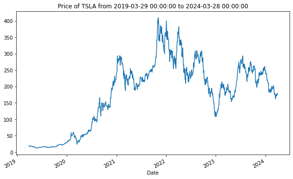
We pull in the values and plot the data. This is a nice looking time series! You can see lots of volatility in the stock which makes it interesting to imagine what will happen next?

Monte Carlo Simulation

We need to set two parameters to run the simulation. One is the number of days we will predict into the future and the other is how many times we will simulate the future. For this project, I set it future date to be the beginning of the next financial quarter.

I like to do 1000 simulations. You can do more but there are diminishing returns as you do more simulations (statistics).

In this code, I use the historic variability of the stock as a constraint for how much the value of the stock can fluctuate from day to day. The python goes through and takes the pervious value to predict the current value. The prediction is based on the Black Scholes method and includes historic volatility plus some randomness.

Geometric Brownian Motion

I assume the log of the returns (percent changes) are normally distributed and that the market is efficient. The formula for the change in price between periods is the price of the stock in t_0 multiplied by the expected drift (average change in price) plus an exogenous shock.

pred_end_date = datetime.datetime(2024, 7, 1)

def monte_carlo(pred_end_date, df=df, iterations=1000, plot=True):
    pred_end_date = pred_end_date
    forecast_dates = [d if d.isoweekday() in range(1, 6) else np.nan for d in pd.date_range(df.index.max(), pred_end_date)] 
    intervals = len(forecast_dates)
    iterations = iterations
    #Preparing log returns from data
    log_returns = np.log(1 + df['Adj Close'].pct_change())

    #Setting up drift and random component in relation to asset data
    u = log_returns.mean()
    var = log_returns.var()
    drift = u - (0.5 * var)
    stdev = log_returns.std()
    daily_returns = np.exp(drift + stdev * norm.ppf(np.random.rand(intervals, iterations)))

    #Takes last data point as startpoint point for simulation

    price_list = np.zeros_like(daily_returns)
    price_list[0] = df['Adj Close'].values[-1]
    #Applies Monte Carlo simulation in asset
    for t in range(1, intervals):
        price_list[t] = price_list[t - 1] * daily_returns[t]

    forecast_df = pd.DataFrame(price_list)
    
    if plot: 
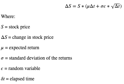
        forecast_df.plot(figsize=(10,6), legend=False, title = "{} Simulated Future Paths".format(iterations))
    
    end_values_df = forecast_df.tail(1)
    
    return forecast_df, end_values_df

forecast_df, end_values_df = monte_carlo(pred_end_date)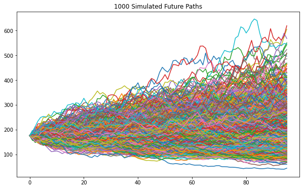

Histogram of final predicted values

The simulated future paths graph is neat but very hard to read. I’m interested in what the price will be on July 1, 2024. So I want to look at the predicted values for that day only and see the distribution of those values.

I can do this with a histogram. The code is based on another project I did for histograms.

Visualizing the normal distribution with Python and Matplotlib

This is a simple python project to show how to simulate a normal distribution and plot it using Matplotlib.

medium.com

I assume the values are normally distributed because of the randomness in the Monte Carlo process.

def plot_norm_hist(s, vline = True, title= True):
    mu, sigma = np.mean(s), np.std(s) # mean and standard deviation

    count, bins, ignored = plt.hist(s, 30, density=True)
    plt.plot(bins, 1/(sigma * np.sqrt(2 * np.pi)) *
               np.exp( - (bins - mu)**2 / (2 * sigma**2) ),
         linewidth=2, color='r')
    
    if vline:
        lline = -.67*sigma + mu
        uline = .67*sigma + mu
        plt.axvline(lline, color='g')
        plt.axvline(uline, color='g')

    if title:
        plt.title("Final price distribution\n Mean: ${:.02f} and Standard Devivation: {:.02f}".format(mu, sigma))
    
    return plt.show()
        
s = end_values_df.iloc[-1]
plot_norm_hist(s, vline=True, title=True)

Now I have a very simple chart and some useful info. The mean value for the stock is $211.43 for July 1, 2024. That is up ~21% from the value from yesterday (March 28, 2024) of $175.79.

So this analysis suggests that the future price will very likely be more than the current price. In fact, this approach predicts the value of Tesla will be high than the current price in 62.8% of the simulations.

Based on this, would you buy the stock today?