
NVIDIA Short-Term Stock Price Forecasting: SHAP Explainer, Lags, Optimized ML Regressors, Auto-ARIMA, Multi-Seasonal FB Prophet Tuning & LSTM

- “Most forecasts don’t allow for alternative outcomes.” Howard Marks.
- The key question is whether the integrated Explainable AI, Statistical Modeling, Supervised ML algorithms and model tuning can predict the future of NVIDIA’s AI with alternative outcomes.
- This article is about NVIDIA (NASDAQ: NVDA) Short-Term Stock Price Forecasting [3] using SHAP 60+ Feature Engineering (FE) [1], Basic Linear Regression with Time Lags [2], 8 Supervised ML Regressors (Scikit-Learn) with Hyperparameter Optimization (HPO) [1,4], Auto-ARIMA time series fitting [1,5], Multi-Seasonal FB Prophet Forecasting HPO with anomalous dates [1], and end-to-end LSTM with Validation QC.
Motivation
- NVIDIA is one of the ‘Magnificent Seven’ group of influential US mega stocks (along with Apple, Microsoft, Alphabet, Amazon, Tesla and Meta Platforms) [3].
- The business has enjoyed meteoric success in recent years and, on 18 June 2024, leap-frogged both Microsoft and Apple to briefly become the world’s most valuable company.
- Charlie Huggins, manager of the Wealth Club Quality Shares Portfolio, says: “The NVIDIA stock split doesn’t change the fundamentals, or value, of the business. But it could make the shares even more attractive to retail investors.”
- Thanks to the boom in AI, NVIDIA is enjoying a purple patch. According to Victoria Scholar, head of investment at interactive investor, an online share trading service, the “AI stock market darling” was the most bought stock among the platform’s UK investors for the second month running in May 2024.
Challenge
- It’s impossible to predict with certainty how a company’s share price will perform [3].
- A stock’s behavior depends partly on the business’s internal performance, combined with wider macro-economic events affecting the markets in which it operates.
Objectives
- Predict short-term NVDA stock price through analyzing the relationship between the stock price and various features.
- Ultimately, the primary goal is to enhance the accuracy of NVDA price predictions, enabling investors to anticipate market movements and potentially maximize profits.
- Including making informed investment decisions, averting losses, optimizing stockholder investments, and improving decision-making strategies.
Tools
The Machine Learning library SciKit-learn in Python comes with a load of features to simplify ML:
- Supervised ML: Generalized linear models such as Linear regression, Decision Trees, SVM, Random Forest, Bayesian methods, etc.
- Unsupervised ML: factoring, clustering, PCA, and unsupervised NN.
- Cross-validation: The accuracy and validity of supervised models on unseen data can be checked with the help of SciKit-learn.
- FB Prophet
Developed by Facebook (FB) and made an open-source contribution to the data science community, Prophet is a powerful forecasting tool available in both R and Python. It is fast, accurate, automated, and feature-rich.
For the time series forecasting shown below, we will be using FB Prophet. More information can be found here: https://facebook.github.io/prophet/
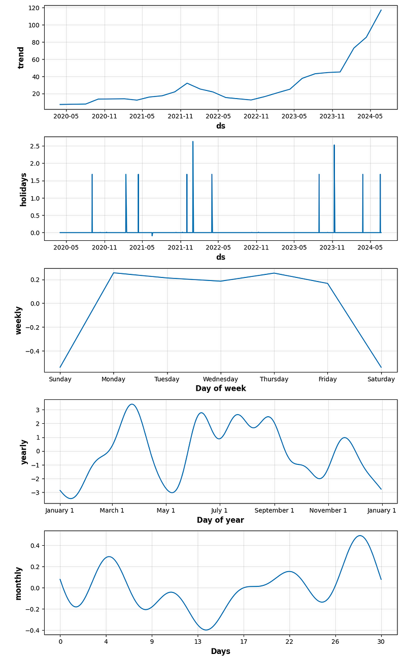
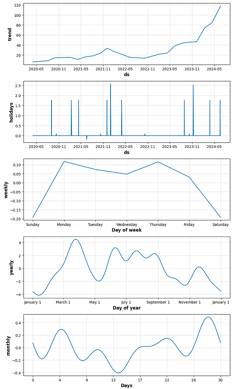
Pros: The model provides an interpretable decomposition of the data that is observed or forecasted into seasonal, trend, and holiday components. This is useful if you want to understand why you are seeing certain patterns on certain day.
Cons: Seasonality not explicitly modeled; lagged effect when forecasting; lacks support for multiple inputs.
ARIMA perform well, if data is not stationary then we can use differencing to make it stationary. If data exhibits clear trends and regular seasonality, ARIMA can be a good choice. ARIMA’s forecasting accuracy tends to reduce as the forecast horizon increases. So it is not good for long-term forecasts.
Read more here.
Using Keras and Tensorflow (TF) makes building NN much easier to build from scratch.
Scikit-Learn is primarily used for traditional ML tasks and algorithms.
TF is mainly utilized for deep learning problems, particularly in AI.
SHAP (SHapley Additive exPlanations) values are a way to explain the output of any machine learning model. It uses a game theoretic approach that measures each player’s contribution to the final outcome. In ML, each feature is assigned an importance value representing its contribution to the model’s output.
SHAP values show how each feature affects each final prediction, the significance of each feature compared to others, and the model’s reliance on the interaction between features.
8 Supervised ML Algorithms
  name                               model
0 Linear Regression                  LinearRegression()
1 KNeighbors Regressor               KNeighborsRegressor()
2 Support Vector Machines            SVR()
3 Linear SVR                         LinearSVR()
4 Random Forest Regressor            RandomForestRegressor()
5 Bagging Regressor                  BaggingRegressor()
6 XGB Regressor                      XGBRegressor()
7 MLP Regressor                      MLPRegressor()
Key ML Error Metrics
- R2 score, RMSE, MAE, Explained Variance Score, and MAPE.
Milestones
- Exploratory Data Analysis (EDA) of Input Stock Data
- Basic Linear Regression with Time-Step & Lag Features
- TSFRESH Feature Engineering [1]
- Multi-Seasonal FB Prophet Prediction & HPO
- Auto-ARIMA Model Fitting & SARIMAX QC Summary
- SciKit-Learn Supervised ML Regression & HPO
- SHAP Feature Dominance Analysis
- TF LSTM Keras Prediction & Validation QC
Let’s get into the specifics of the proposed methodology with a final source code line-by-line explained.
Python Imports, Installations & Settings
- Installing/importing necessary Python libraries and setting parameters
!pip install seaborn, yfinance, sklearn, tsfresh, prophet, lightgbm, xgboost, pmdarima, shap, statsmodels, plotly, xgboost

import random
import os
import numpy as np
import pandas as pd
import requests
#import pandas_datareader as web
import yfinance as yf

# Date
import datetime as dt
from datetime import date, timedelta, datetime

# EDA
import seaborn as sns
import matplotlib.pyplot as plt
from matplotlib.pylab import rcParams
import plotly.express as px
import plotly.graph_objects as go
from plotly.offline import init_notebook_mode
init_notebook_mode(connected=True)

# FE
from tsfresh import extract_features, select_features, extract_relevant_features
from tsfresh.utilities.dataframe_functions import impute
from sklearn.inspection import permutation_importance

import shap

# Time Series Modelling
import statsmodels.api as sm
from statsmodels.graphics.tsaplots import plot_acf, plot_pacf
from statsmodels.tsa.stattools import adfuller
from statsmodels.tsa.seasonal import seasonal_decompose
from statsmodels.tsa.arima_model import ARIMA

# Metrics
from sklearn.metrics import r2_score
from sklearn.metrics import mean_squared_error, mean_absolute_percentage_error

# Modeling and preprocessing
from sklearn.preprocessing import StandardScaler, MinMaxScaler
from sklearn.model_selection import train_test_split, GridSearchCV
from sklearn.linear_model import LinearRegression
from sklearn.svm import SVR, LinearSVR
from sklearn.neighbors import KNeighborsRegressor
from sklearn.ensemble import RandomForestRegressor
from sklearn.ensemble import BaggingRegressor, AdaBoostRegressor
from sklearn.neural_network import MLPRegressor
from prophet import Prophet
import xgboost as xgb
from xgboost import XGBRegressor
import lightgbm as lgb
from lightgbm import LGBMRegressor
import pmdarima as pm

import warnings
warnings.filterwarnings("ignore")

# Set random state
def fix_all_seeds(seed):
    np.random.seed(seed)
    random.seed(seed)
    os.environ['PYTHONHASHSEED'] = str(seed)

random_state = 42
fix_all_seeds(random_state)


# Set main parameters
cryptocurrency = 'NVDA' #define any stock
target = 'Close'
forecasting_days = 10

# Set time interval of data for given cryptocurrency - the period of coronavirus in 2020-2021
date_start = dt.datetime(2020, 4, 1)
# date_end = dt.datetime.now()
date_end = dt.datetime(2024, 7, 13)
Reading & Analyzing Input Stock Data
- Using Yahoo Finance to fetch the daily NVIDIA historical data from 2020–04–01 to 2024–07–12
def get_data(cryptocurrency, date_start, date_end=None):
    # Get data for a given stock
    # date_end = None means that the date_end is the current day

    if date_end is None:
        date_end = dt.datetime.now()

    df =yf.download(cryptocurrency, date_start, date_end)

    return df

# Download data of the cryptocurrency via API
df = get_data(cryptocurrency, date_start, date_end)- Let’s drop ‘Adj Close’ and take a look at the general structure, descriptive statistics of the dataset and missing values if any
df = df.drop(columns = ["Adj Close"])
df.tail()

           Open       High       Low        Close      Volume
Date
2024-07-08 127.489998 130.770004 127.040001 128.199997 237677300
2024-07-09 130.350006 133.820007 128.649994 131.380005 285366600
2024-07-10 134.029999 135.100006 132.419998 134.910004 248978600
2024-07-11 135.750000 136.149994 127.050003 127.400002 374782700
2024-07-12 128.259995 131.919998 127.220001 129.240005 252103100

df.shape
(1077, 5)

df.info()

<class 'pandas.core.frame.DataFrame'>
DatetimeIndex: 1077 entries, 2020-04-01 to 2024-07-12
Data columns (total 5 columns):
 #   Column  Non-Null Count  Dtype
---  ------  --------------  -----
 0   Open    1077 non-null   float64
 1   High    1077 non-null   float64
 2   Low     1077 non-null   float64
 3   Close   1077 non-null   float64
 4   Volume  1077 non-null   int64
dtypes: float64(4), int64(1)
memory usage: 50.5 KB

df_nan_count = df.isna().sum()

print(df_nan_count)
Open      0
High      0
Low       0
Close     0
Volume    0
dtype: int64- Creating the column ‘Time’ as follows
df['Time'] = np.arange(len(df.index))

Date
2020-01-02       0
2020-01-03       1
2020-01-06       2
2020-01-07       3
2020-01-08       4
              ...
2024-07-08    1134
2024-07-09    1135
2024-07-10    1136
2024-07-11    1137
2024-07-12    1138
Name: Time, Length: 1139, dtype: int32- Using Plotly to plot the interactive stock candlesticks
import pandas as pd
import plotly.io as pio
import plotly.graph_objects as go
pio.renderers.default='browser'

def get_candlestick_chart(df: pd.DataFrame):

    layout = go.Layout(
        title = 'NVDA Stock Price',
        xaxis = {'title': 'Date'},
        yaxis = {'title': 'Price'},
    )

    fig = go.Figure(
        layout=layout,
        data=[
            go.Candlestick(
                x = df['Date'],
                open = df['Open'],
                high = df['High'],
                low = df['Low'],
                close = df['Close'],
                name = 'Candlestick chart'
            ),
        ]
    )

    fig.update_xaxes(rangebreaks = [{'bounds': ['sat', 'mon']}])

    return fig

if __name__ == '__main__':
    fig = get_candlestick_chart(df)
    fig.show()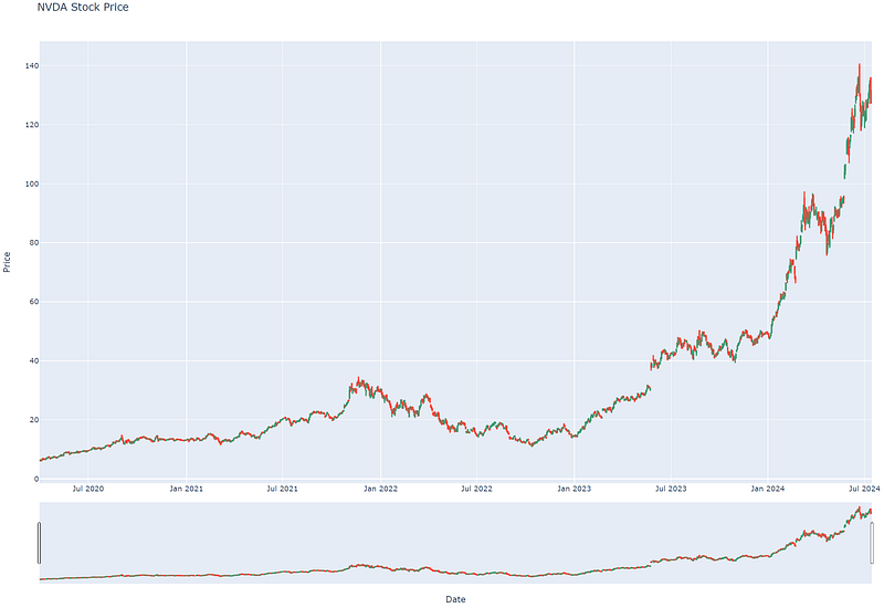
Linear Regression with Time-Step & Lag Features
- Let’s begin with Linear Regression (LR) using the most basic time-step feature ‘Time’ v.s. (aka time dummy)
#import matplotlib.pyplot as plt
#import seaborn as sns

plt.rc(
    "figure",
    autolayout=True,
    figsize=(11, 4),
    titlesize=18,
    titleweight='bold',
)
plt.rc(
    "axes",
    labelweight="bold",
    labelsize="large",
    titleweight="bold",
    titlesize=16,
    titlepad=10,
)
%config InlineBackend.figure_format = 'retina'

fig, ax = plt.subplots()
ax.plot('Time', 'Close', data=df, color='0.75')
ax = sns.regplot(x='Time', y='Close', data=df, ci=None, scatter_kws=dict(color='0.25'))
ax.set_title('Linear Regression of NVDA Price vs Time Dummy');
plt.grid()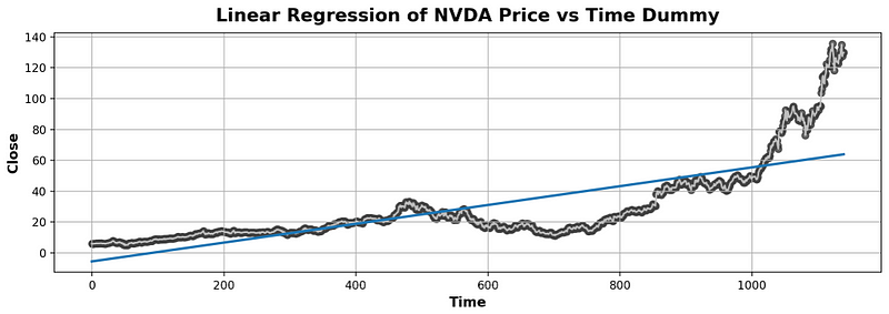
- Clearly, LR does not fit the Close price well as Time>1000.
- Let’s try LR with lag features [2].
- Firstly, we compute Lag_10 for the 10-day forecast
df['Lag_10'] = df['Close'].shift(10)
df = df.reindex(columns=['Close', 'Lag_10'])

#df.head()

fig, ax = plt.subplots()
ax = sns.regplot(x='Lag_10', y='Close', data=df, ci=None, scatter_kws=dict(color='0.25'))
ax.set_aspect('equal')
ax.set_title('Lag-10 X-Plot of NVDA Price');
plt.grid()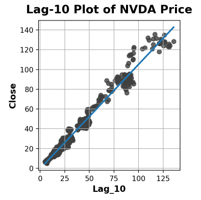
- Training the LR model with the above feature and making predictions
from sklearn.linear_model import LinearRegression

# Training data
X = df.loc[:, ['Lag_10']].fillna(method='bfill')  # features
y = df.loc[:, 'Close']  # target

# Train the model
model = LinearRegression()
model.fit(X, y)

# Store the fitted values as a time series with the same time index as
# the training data
y_pred = pd.Series(model.predict(X), index=X.index)

y.plot(label='Close')
y_pred.plot(label='LR Lag_10')
plt.legend()
plt.title('NVDA Close Price vs LR Lag_10')
plt.grid()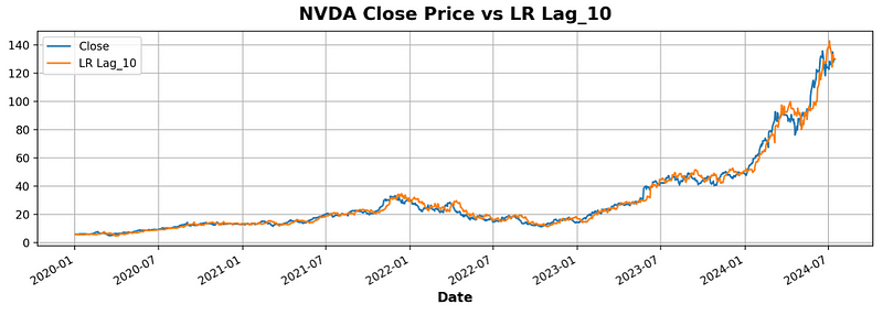
- Quantifying the quality of LR predictions
from sklearn.metrics import r2_score
r2_score(y, y_pred)
0.9806962531842807

from sklearn.metrics import root_mean_squared_error
root_mean_squared_error(y, y_pred)
3.62088252156672

from sklearn.metrics import mean_absolute_error
mean_absolute_error(y, y_pred)
2.2952125909109022

from sklearn.metrics import explained_variance_score
explained_variance_score(y, y_pred)
0.9806962531842807
TSFRESH Feature Engineering
- Performing Feature Engineering with TSFRESH [1]
def get_tsfresh_features(data):
    # Get statistic features using library TSFRESH
    # Thanks to https://www.kaggle.com/code/vbmokin/btc-growth-forecasting-with-advanced-fe-for-ohlc

    data = data.reset_index(drop=False).reset_index(drop=False)

    # Extract features
    extracted_features = extract_features(data, column_id="Date", column_sort="Date")

    # Drop features with NaN
    extracted_features_clean = extracted_features.dropna(axis=1, how='all').reset_index(drop=True)

    # Drop features with constants
    cols_std_zero  = []
    for col in extracted_features_clean.columns:
        if extracted_features_clean[col].std()==0:
            cols_std_zero.append(col)
    extracted_features_clean = extracted_features_clean.drop(columns = cols_std_zero)

    extracted_features_clean['Date'] = data['Date']   # For the merging

    return extracted_features_clean

extracted_features_clean = get_tsfresh_features(df[['Close']])
#extracted_features_clean

extracted_features_clean.info()

<class 'pandas.core.frame.DataFrame'>
RangeIndex: 1077 entries, 0 to 1076
Data columns (total 51 columns):
 #   Column                                                         Non-Null Count  Dtype
---  ------                                                         --------------  -----
 0   index__sum_values                                              1077 non-null   float64
 1   index__abs_energy                                              1077 non-null   float64
 2   index__median                                                  1077 non-null   float64
 3   index__mean                                                    1077 non-null   float64
 4   index__root_mean_square                                        1077 non-null   float64
 5   index__maximum                                                 1077 non-null   float64
 6   index__absolute_maximum                                        1077 non-null   float64
 7   index__minimum                                                 1077 non-null   float64
 8   index__benford_correlation                                     1076 non-null   float64
 9   index__quantile__q_0.1                                         1077 non-null   float64
 10  index__quantile__q_0.2                                         1077 non-null   float64
 11  index__quantile__q_0.3                                         1077 non-null   float64
 12  index__quantile__q_0.4                                         1077 non-null   float64
 13  index__quantile__q_0.6                                         1077 non-null   float64
 14  index__quantile__q_0.7                                         1077 non-null   float64
 15  index__quantile__q_0.8                                         1077 non-null   float64
 16  index__quantile__q_0.9                                         1077 non-null   float64
 17  index__cwt_coefficients__coeff_0__w_2__widths_(2, 5, 10, 20)   1077 non-null   float64
 18  index__cwt_coefficients__coeff_0__w_5__widths_(2, 5, 10, 20)   1077 non-null   float64
 19  index__cwt_coefficients__coeff_0__w_10__widths_(2, 5, 10, 20)  1077 non-null   float64
 20  index__cwt_coefficients__coeff_0__w_20__widths_(2, 5, 10, 20)  1077 non-null   float64
 21  index__fft_coefficient__attr_"real"__coeff_0                   1077 non-null   float64
 22  index__fft_coefficient__attr_"abs"__coeff_0                    1077 non-null   float64
 23  index__value_count__value_0                                    1077 non-null   float64
 24  index__value_count__value_1                                    1077 non-null   float64
 25  index__range_count__max_1__min_-1                              1077 non-null   float64
 26  index__count_below__t_0                                        1077 non-null   float64
 27  Close__sum_values                                              1077 non-null   float64
 28  Close__abs_energy                                              1077 non-null   float64
 29  Close__median                                                  1077 non-null   float64
 30  Close__mean                                                    1077 non-null   float64
 31  Close__root_mean_square                                        1077 non-null   float64
 32  Close__maximum                                                 1077 non-null   float64
 33  Close__absolute_maximum                                        1077 non-null   float64
 34  Close__minimum                                                 1077 non-null   float64
 35  Close__benford_correlation                                     1077 non-null   float64
 36  Close__quantile__q_0.1                                         1077 non-null   float64
 37  Close__quantile__q_0.2                                         1077 non-null   float64
 38  Close__quantile__q_0.3                                         1077 non-null   float64
 39  Close__quantile__q_0.4                                         1077 non-null   float64
 40  Close__quantile__q_0.6                                         1077 non-null   float64
 41  Close__quantile__q_0.7                                         1077 non-null   float64
 42  Close__quantile__q_0.8                                         1077 non-null   float64
 43  Close__quantile__q_0.9                                         1077 non-null   float64
 44  Close__cwt_coefficients__coeff_0__w_2__widths_(2, 5, 10, 20)   1077 non-null   float64
 45  Close__cwt_coefficients__coeff_0__w_5__widths_(2, 5, 10, 20)   1077 non-null   float64
 46  Close__cwt_coefficients__coeff_0__w_10__widths_(2, 5, 10, 20)  1077 non-null   float64
 47  Close__cwt_coefficients__coeff_0__w_20__widths_(2, 5, 10, 20)  1077 non-null   float64
 48  Close__fft_coefficient__attr_"real"__coeff_0                   1077 non-null   float64
 49  Close__fft_coefficient__attr_"abs"__coeff_0                    1077 non-null   float64
 50  Date                                                           1077 non-null   datetime64[ns]
dtypes: datetime64[ns](1), float64(50)
memory usage: 429.2 KB- Merging all features
df = pd.merge(df, extracted_features_clean, how='left', on='Date')

df.shape
(1077, 56)- Adding more features
def get_add_features(df_feat):
    # FE for data as row of DataFrame
    # Thanks to https://www.kaggle.com/code/vbmokin/g-research-crypto-forecasting-baseline-fe

    # Two new features from the competition tutorial
    df_feat['Upper_Shadow'] = df_feat['High'] - np.maximum(df_feat['Close'], df_feat['Open'])
    df_feat['Lower_Shadow'] = np.minimum(df_feat['Close'], df_feat['Open']) - df_feat['Low']

    # Thanks to https://www.kaggle.com/code1110/gresearch-simple-lgb-starter
    df_feat['lower_shadow'] = np.minimum(df_feat['Close'], df_feat['Open']) - df_feat['Low']
    df_feat['high2low'] = (df_feat['High'] / df_feat['Low']).replace([np.inf, -np.inf, np.nan], 0.)

    return df_feat

df = get_add_features(df)
df.info()

<class 'pandas.core.frame.DataFrame'>
RangeIndex: 1077 entries, 0 to 1076
Data columns (total 60 columns):
 #   Column                                                         Non-Null Count  Dtype
---  ------                                                         --------------  -----
 0   Date                                                           1077 non-null   datetime64[ns]
 1   Open                                                           1077 non-null   float64
 2   High                                                           1077 non-null   float64
 3   Low                                                            1077 non-null   float64
 4   Close                                                          1077 non-null   float64
 5   Volume                                                         1077 non-null   int64
 6   index__sum_values                                              1077 non-null   float64
 7   index__abs_energy                                              1077 non-null   float64
 8   index__median                                                  1077 non-null   float64
 9   index__mean                                                    1077 non-null   float64
 10  index__root_mean_square                                        1077 non-null   float64
 11  index__maximum                                                 1077 non-null   float64
 12  index__absolute_maximum                                        1077 non-null   float64
 13  index__minimum                                                 1077 non-null   float64
 14  index__benford_correlation                                     1076 non-null   float64
 15  index__quantile__q_0.1                                         1077 non-null   float64
 16  index__quantile__q_0.2                                         1077 non-null   float64
 17  index__quantile__q_0.3                                         1077 non-null   float64
 18  index__quantile__q_0.4                                         1077 non-null   float64
 19  index__quantile__q_0.6                                         1077 non-null   float64
 20  index__quantile__q_0.7                                         1077 non-null   float64
 21  index__quantile__q_0.8                                         1077 non-null   float64
 22  index__quantile__q_0.9                                         1077 non-null   float64
 23  index__cwt_coefficients__coeff_0__w_2__widths_(2, 5, 10, 20)   1077 non-null   float64
 24  index__cwt_coefficients__coeff_0__w_5__widths_(2, 5, 10, 20)   1077 non-null   float64
 25  index__cwt_coefficients__coeff_0__w_10__widths_(2, 5, 10, 20)  1077 non-null   float64
 26  index__cwt_coefficients__coeff_0__w_20__widths_(2, 5, 10, 20)  1077 non-null   float64
 27  index__fft_coefficient__attr_"real"__coeff_0                   1077 non-null   float64
 28  index__fft_coefficient__attr_"abs"__coeff_0                    1077 non-null   float64
 29  index__value_count__value_0                                    1077 non-null   float64
 30  index__value_count__value_1                                    1077 non-null   float64
 31  index__range_count__max_1__min_-1                              1077 non-null   float64
 32  index__count_below__t_0                                        1077 non-null   float64
 33  Close__sum_values                                              1077 non-null   float64
 34  Close__abs_energy                                              1077 non-null   float64
 35  Close__median                                                  1077 non-null   float64
 36  Close__mean                                                    1077 non-null   float64
 37  Close__root_mean_square                                        1077 non-null   float64
 38  Close__maximum                                                 1077 non-null   float64
 39  Close__absolute_maximum                                        1077 non-null   float64
 40  Close__minimum                                                 1077 non-null   float64
 41  Close__benford_correlation                                     1077 non-null   float64
 42  Close__quantile__q_0.1                                         1077 non-null   float64
 43  Close__quantile__q_0.2                                         1077 non-null   float64
 44  Close__quantile__q_0.3                                         1077 non-null   float64
 45  Close__quantile__q_0.4                                         1077 non-null   float64
 46  Close__quantile__q_0.6                                         1077 non-null   float64
 47  Close__quantile__q_0.7                                         1077 non-null   float64
 48  Close__quantile__q_0.8                                         1077 non-null   float64
 49  Close__quantile__q_0.9                                         1077 non-null   float64
 50  Close__cwt_coefficients__coeff_0__w_2__widths_(2, 5, 10, 20)   1077 non-null   float64
 51  Close__cwt_coefficients__coeff_0__w_5__widths_(2, 5, 10, 20)   1077 non-null   float64
 52  Close__cwt_coefficients__coeff_0__w_10__widths_(2, 5, 10, 20)  1077 non-null   float64
 53  Close__cwt_coefficients__coeff_0__w_20__widths_(2, 5, 10, 20)  1077 non-null   float64
 54  Close__fft_coefficient__attr_"real"__coeff_0                   1077 non-null   float64
 55  Close__fft_coefficient__attr_"abs"__coeff_0                    1077 non-null   float64
 56  Upper_Shadow                                                   1077 non-null   float64
 57  Lower_Shadow                                                   1077 non-null   float64
 58  lower_shadow                                                   1077 non-null   float64
 59  high2low                                                       1077 non-null   float64
dtypes: datetime64[ns](1), float64(58), int64(1)
memory usage: 505.0 KB
FB Prophet Prediction
- Preparing the DF for FB Prophet forecasting [1]
# Create a new dataframe with anomalous dates for Facebook Prophet
if is_anomalies:
anomalous_dates = ['2020-09-03', '2021-02-12', '2021-04-13', '2021-12-02',
'2022-04-01', '2023-08-29', '2024-03-26', '2024-06-18']
holidays_df = pd.DataFrame(columns = ['ds', 'lower_window', 'upper_window', 'prior_scale'])
holidays_df['ds'] = anomalous_dates
holidays_df['holiday'] = 'anomalous_dates'
holidays_df['lower_window'] = 0
holidays_df['upper_window'] = 0
holidays_df['prior_scale'] = 10
display(holidays_df)
ds lower_window upper_window prior_scale holiday
0 2020-09-03 0 0 10 anomalous_dates
1 2021-02-12 0 0 10 anomalous_dates
2 2021-04-13 0 0 10 anomalous_dates
3 2021-12-02 0 0 10 anomalous_dates
4 2022-04-01 0 0 10 anomalous_dates
5 2023-08-29 0 0 10 anomalous_dates
6 2024-03-26 0 0 10 anomalous_dates
7 2024-06-18 0 0 10 anomalous_dates
# Add a few more anomalous dates
if is_anomalies:
anomalous_dates_diff = anomalous_dates.copy()
anomalous_dates_diff.append('2022-08-08')
anomalous_dates_diff.append('2022-12-01')
anomalous_dates_diff.append('2023-11-21')
print(anomalous_dates_diff)
['2020-09-03', '2021-02-12', '2021-04-13', '2021-12-02', '2022-04-01', '2023-08-29', '2024-03-26', '2024-06-18', '2022-08-08', '2022-12-01', '2023-11-21']
# Create a new feature in df for anomalous_dates_diff
if is_anomalies:
df['Close_diff_anomalous'] = df['Date'].isin(anomalous_dates_diff).astype('int')
display(df)
# Number of anomalous dates
print(f"Number of anomalous dates - {df['Close_diff_anomalous'].sum()}")
Number of anomalous dates - 11
# Illustration of number transformations in the columns:
# "Close" -> "Close_diff" -> "Target" -> "Close_diff_pred" -> "Close_pred"
# Get target and the result of the forecasting
forecasting_days_example = 3
df_example = pd.DataFrame({'Close':[1, 2, 4, 8, 15, 25], 'Day': [0, 1, 2, 3, 4, 5]})
df_example['Close_diff'] = df_example['Close'].diff()
df_example['target'] = df_example['Close_diff'].shift(-forecasting_days_example)
df_example['target_pred'] = df_example['target'].copy() # Ideal forecasting result
print(f'Simulation of the result of ideal forecasting the "target_pred" for {forecasting_days_example} days')
display(df_example[['Day', 'Close', 'Close_diff', 'target', 'target_pred']])
# Get inverse target
print('\nSimulation of the recovering predicted values "Close_pred" from the "target_pred"')
df_example['Close_diff_pred_shifted'] = df_example['target_pred'].shift(forecasting_days_example)
# Let's create an intermediate feature to make it easier to explain the transformation
temp_column_name = f'Close_diff_pred_shifted_with_Close' # Intermediate feature for transformations
df_example[temp_column_name] = df_example['Close_diff_pred_shifted'].copy()
df_example.loc[forecasting_days_example, temp_column_name] = df_example.loc[forecasting_days_example,'Close']
df_example['Close_pred'] = np.concatenate((df_example['Close'].tolist()[:forecasting_days_example],
np.cumsum(df_example[temp_column_name].values[forecasting_days_example:], dtype=float)))
df_example['Close_pred'] = df_example['Close_pred'].astype('int')
display(df_example[['Day', 'Close', 'Close_diff', 'target', 'target_pred', 'Close_diff_pred_shifted', temp_column_name, 'Close_pred']])
Simulation of the result of ideal forecasting the "target_pred" for 3 days
Day Close Close_diff target target_pred
0 0 1 NaN 4.0 4.0
1 1 2 1.0 7.0 7.0
2 2 4 2.0 10.0 10.0
3 3 8 4.0 NaN NaN
4 4 15 7.0 NaN NaN
5 5 25 10.0 NaN NaN
Simulation of the recovering predicted values "Close_pred" from the "target_pred"
Day Close Close_diff target target_pred Close_diff_pred_shifted Close_diff_pred_shifted_with_Close Close_pred
0 0 1 NaN 4.0 4.0 NaN NaN 1
1 1 2 1.0 7.0 7.0 NaN NaN 2
2 2 4 2.0 10.0 10.0 NaN NaN 4
3 3 8 4.0 NaN NaN 4.0 8.0 8
4 4 15 7.0 NaN NaN 7.0 7.0 15
5 5 25 10.0 NaN NaN 10.0 10.0 25
def cut_data(df, y, num_start, num_end):
# Cutting dataframe df and array or list for [num_start, num_end-1]
df2 = df[num_start:(num_end+1)]
y2 = y[num_start:(num_end+1)] if y is not None else None
return df2, y2
def get_train_valid_test_ts(df, forecasting_days, target='Close'):
# Get training, validation and test datasets with target for Time Series models
# Data prepairing
df = df.dropna(how="any").reset_index(drop=True)
df = df[['Date', 'Close']]
df.columns = ['ds', 'y']
y = None
N = len(df)
train, _ = cut_data(df, y, 0, N-2*forecasting_days-1)
valid, _ = cut_data(df, y, N-2*forecasting_days, N-forecasting_days-1)
test, _ = cut_data(df, y, N-forecasting_days, N)
# Train+valid - for optimal model training
train_valid = pd.concat([train, valid])
print(f'Origin dataset has {len(df)} rows and {len(df.columns)} features')
print(f'Get training dataset with {len(train)} rows')
print(f'Get validation dataset with {len(valid)} rows')
print(f'Get test dataset with {len(test)} rows')
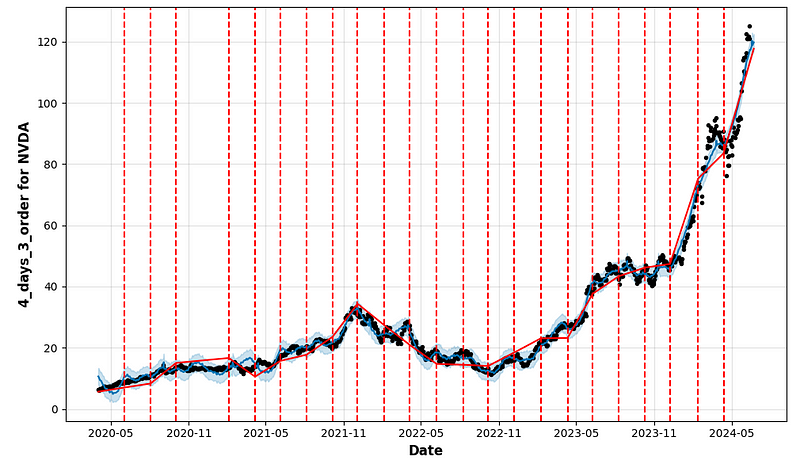
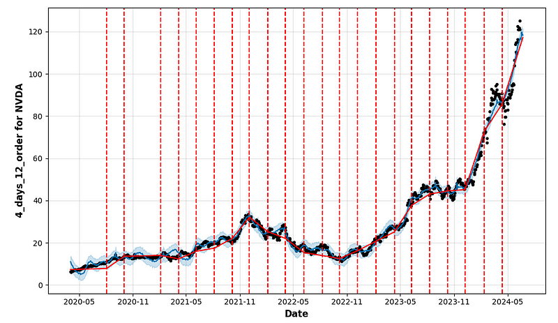
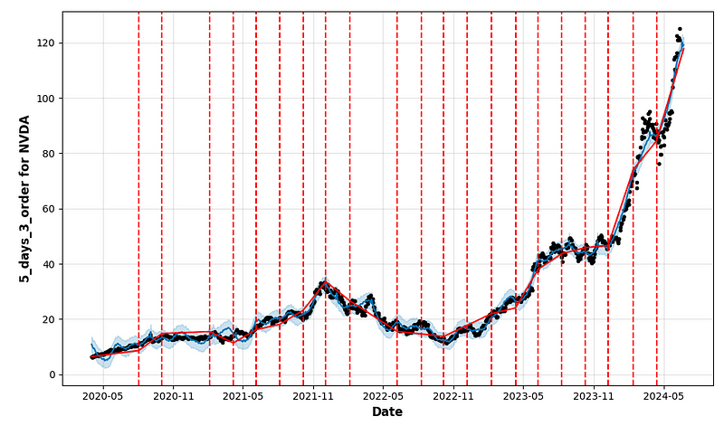
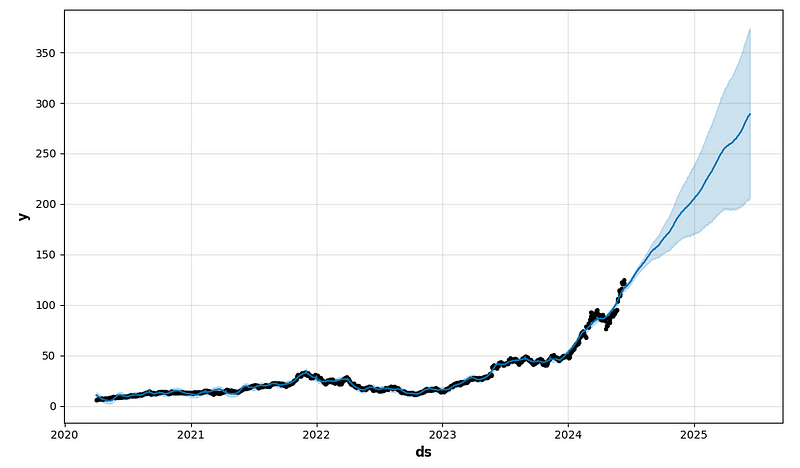
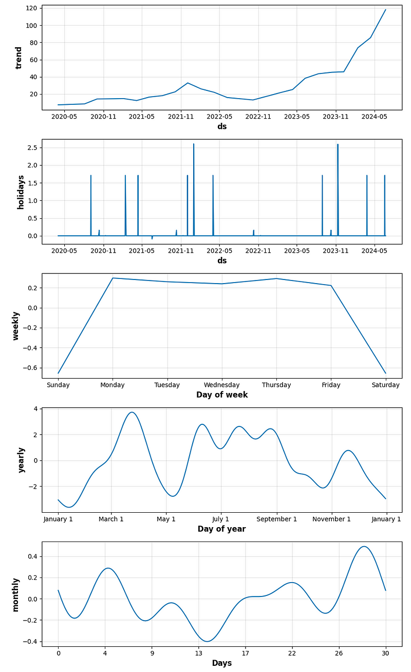
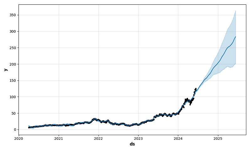
return train, valid, test, train_valid- FB Prophet model training, tuning and forecasting with multiple trends [1], seasonality, the above anomalous dates and in-built US holidays
def get_train_valid_test_mf(df, forecasting_days, target='target'):
# Get training, validation and test datasets with target for multi-features ML models
df = df.drop(columns = ['Date']).dropna(how="any").reset_index(drop=True)
# Save and drop target
y = df.pop(target)
# Get starting points for the recovering "Close" from "Close_diff_shigted"
N = len(df)
#print(f"Total - {N}, Valid start index = {N-forecasting_days-1}, Test start index = {N-1}")
start_points = {'valid_start_point' : df.loc[N-forecasting_days-1, 'Close'],
'test_start_point' : df.loc[N-1, 'Close']}
# Standartization data
scaler = StandardScaler()
df = pd.DataFrame(scaler.fit_transform(df), columns = df.columns)
train, ytrain = cut_data(df.copy(), y, 0, N-2*forecasting_days-1)
valid, yvalid = cut_data(df.copy(), y, N-2*forecasting_days, N-forecasting_days-1)
test, ytest = cut_data(df.copy(), y, N-forecasting_days, N)
# Train+valid - for optimal model training
train_valid = pd.concat([train, valid])
y_train_valid = pd.concat([ytrain, yvalid])
print(f'Origin dataset has {len(df)} rows and {len(df.columns)} features')
print(f'Get training dataset with {len(train)} rows')
print(f'Get validation dataset with {len(valid)} rows')
print(f'Get test dataset with {len(test)} rows')
return train, ytrain, valid, yvalid, test, ytest, train_valid, y_train_valid, start_points
#Model training and forecasting
def calc_metrics(type_score, list_true, list_pred):
# Calculation score with type=type_score for list_true and list_pred
if type_score=='r2_score':
score = r2_score(list_true, list_pred)
elif type_score=='rmse':
score = mean_squared_error(list_true, list_pred, squared=False)
elif type_score=='mape':
score = mean_absolute_percentage_error(list_true, list_pred)
return score
def result_add_metrics(result, n, y_true, y_pred):
# Calculate and add metrics to dataframe result[n,:]
result.loc[n,'r2_score'] = calc_metrics('r2_score', y_true, y_pred)
result.loc[n,'rmse'] = calc_metrics('rmse', y_true, y_pred) # in coins
result.loc[n,'mape'] = 100*calc_metrics('mape', y_true, y_pred) # in %
return result
# Results of all models
result = pd.DataFrame(columns = ['name_model', 'type_data', 'r2_score', 'rmse', 'mape', 'params', 'ypred'])
if is_Prophet:
df2=df.copy()
display(df2)
# Get datasets
if is_Prophet:
train_ts, valid_ts, test_ts, train_valid_ts = get_train_valid_test_ts(df2.copy(), forecasting_days, target='Close')
if not is_anomalies:
holidays_df = None
from prophet.plot import add_changepoints_to_plot
def prophet_modeling(result,
cryptocurrency,
train,
test,
holidays_df,
period_days,
fourier_order_seasonality,
forecasting_period,
name_model,
type_data):
# Performs FB Prophet model training for given train dataset, holidays_df and seasonality_mode
# Performs forecasting with period by this model, visualization and error estimation
# df - dataframe with real data in the forecasting_period
# can be such combinations of parameters: train=train, test=valid or train=train_valid, test=test
# Save results into dataframe result
# Build Prophet model with parameters and structure
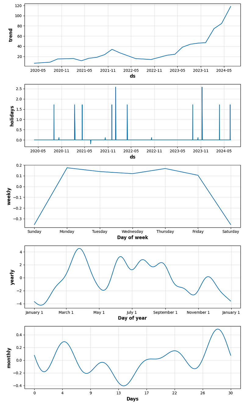
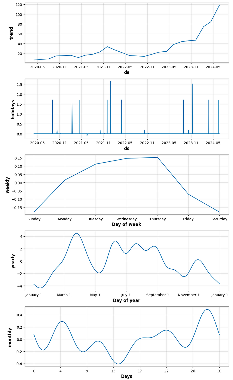
model = Prophet(daily_seasonality=False,
weekly_seasonality=True,
yearly_seasonality=True,
changepoint_range=1,
changepoint_prior_scale = 0.5,
holidays=holidays_df,
seasonality_mode = 'additive'
)
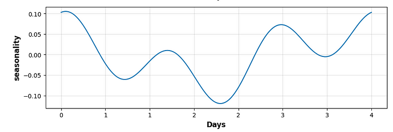
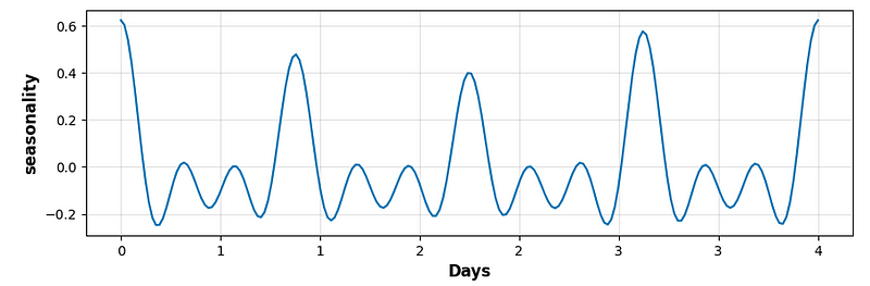
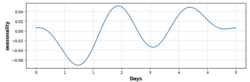
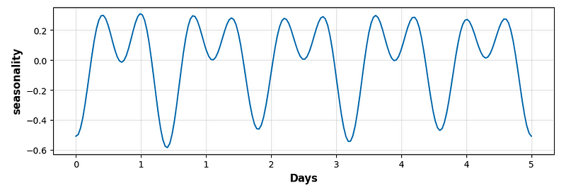
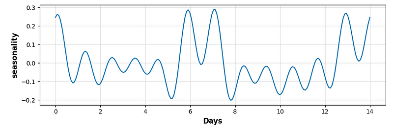
model.add_seasonality(name='seasonality', period=period_days,
fourier_order=fourier_order_seasonality,
mode = 'additive', prior_scale = 0.5)
model.add_seasonality(name='monthly', period=30.5, fourier_order=5)
model.add_country_holidays(country_name='US')
# Training model for df
model.fit(train)
# Make a forecast
future = model.make_future_dataframe(periods = forecasting_period)
forecast = model.predict(future)
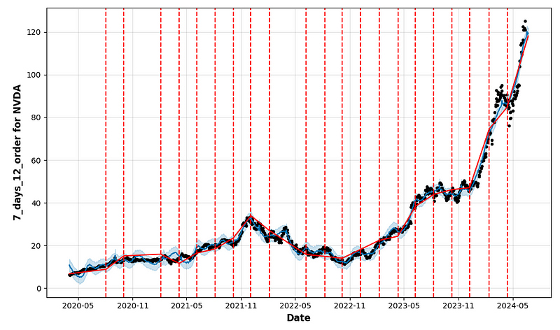
# Draw plot of the values with forecasting data
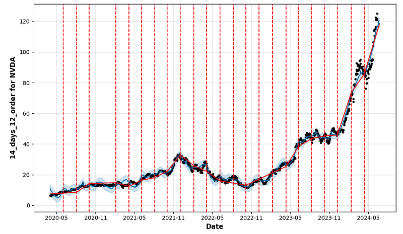
figure = model.plot(forecast, xlabel = 'Date', ylabel = f"{name_model} for {cryptocurrency}")
a = add_changepoints_to_plot(figure.gca(), model, forecast)
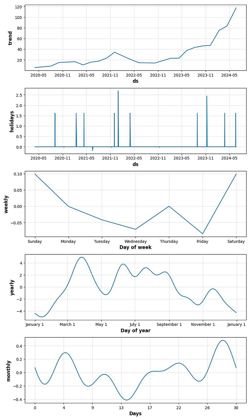
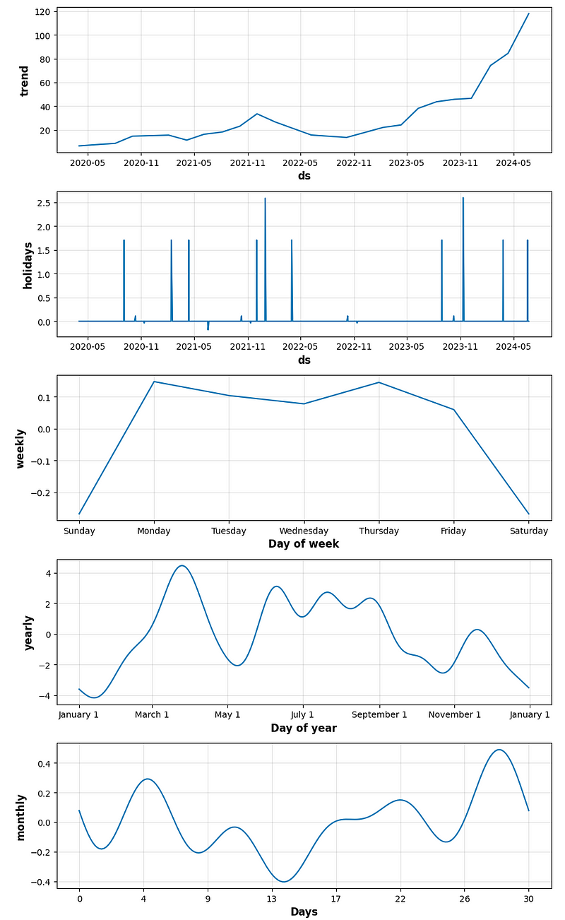
# Draw plot with the components (trend and seasonalities) of the forecasts
figure_component = model.plot_components(forecast)
# Ouput the prediction for the next time on forecasted_days
#forecast[['yhat_lower', 'yhat', 'yhat_upper']] = forecast[['yhat_lower', 'yhat', 'yhat_upper']].round(1)
#forecast[['ds', 'yhat_lower', 'yhat', 'yhat_upper']].tail(forecasting_period)
# Forecasting data by the model
ypred = forecast['yhat'][-forecasting_period:]
#print(ypred)
# Save results
n = len(result)
result.loc[n,'name_model'] = f"Prophet_{name_model}"
result.loc[n,'type_data'] = type_data
result.at[n,'params'] = [period_days]+[fourier_order_seasonality]
result.at[n,'ypred'] = ypred
#result = result_add_metrics(result, n, test['y'], y_pred)
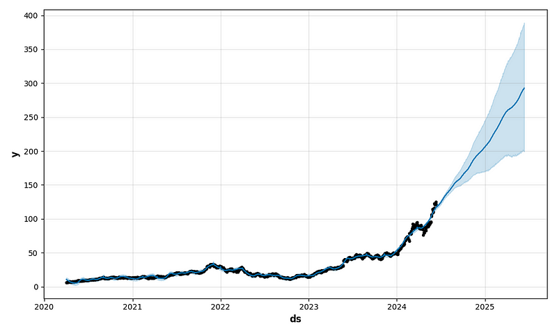
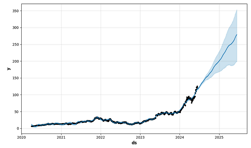
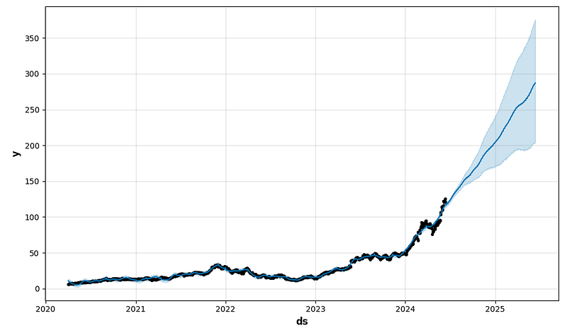
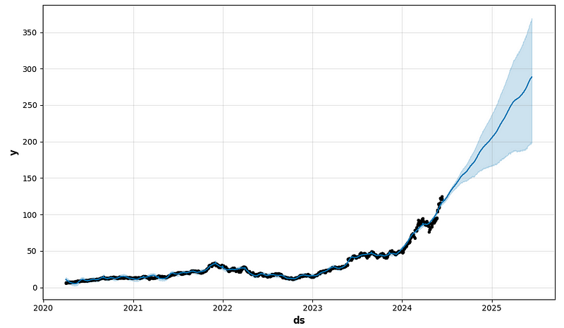
future1 = model.make_future_dataframe(periods=365)
forecast1 = model.predict(future1)
fig1 = model.plot(forecast1)
return result, ypred
# Models tuning
if is_Prophet:
for period_days in [4, 5, 7, 14]:
for fourier_order_seasonality in [3, 12]:
result, _ = prophet_modeling(result,
cryptocurrency,
train_ts,
valid_ts,
holidays_df,
period_days,
fourier_order_seasonality,
forecasting_days,
f'{period_days}_days_{fourier_order_seasonality}_order',
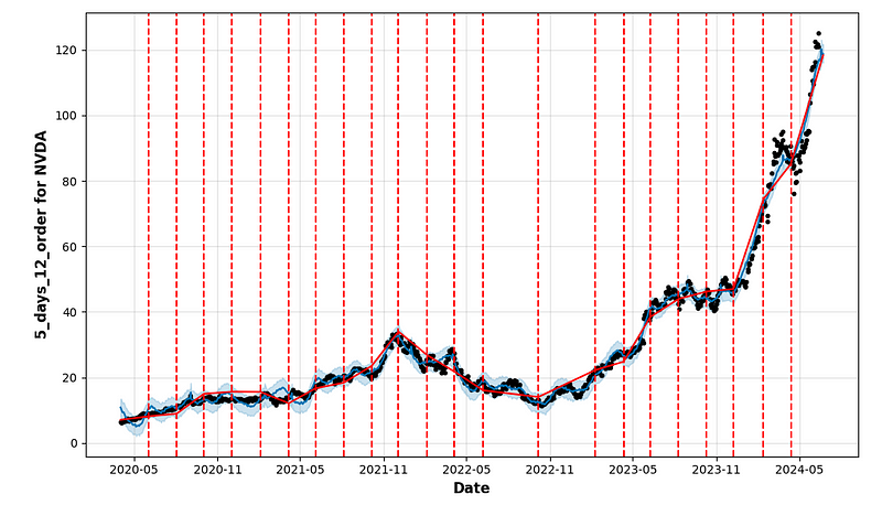
'valid')- Plotting the complete output of FB Prophet forecasting HPO
- period_days=4 & fourier_order_seasonality=3
- period_days=4 & fourier_order_seasonality=12
- period_days=5 & fourier_order_seasonality=3

- period_days=5 & fourier_order_seasonality=12

- period_days=7 & fourier_order_seasonality=3
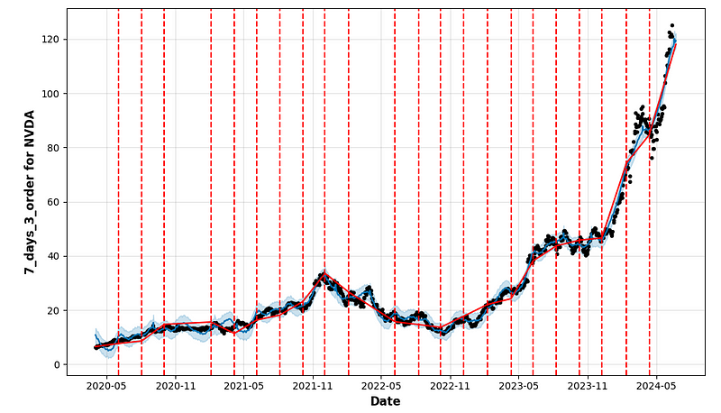
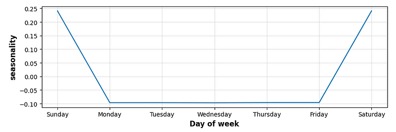
- period_days=7 & fourier_order_seasonality=12
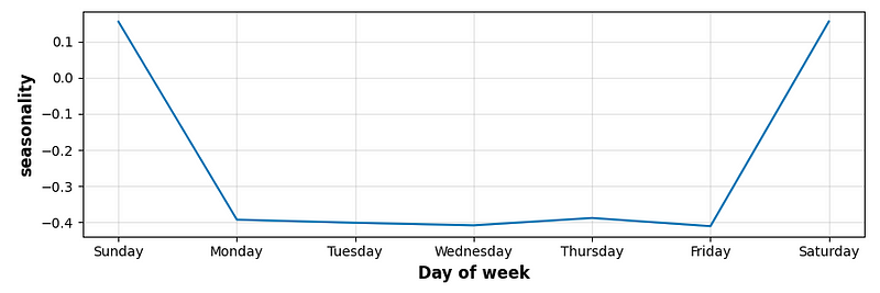

- period_days=14 & fourier_order_seasonality=3
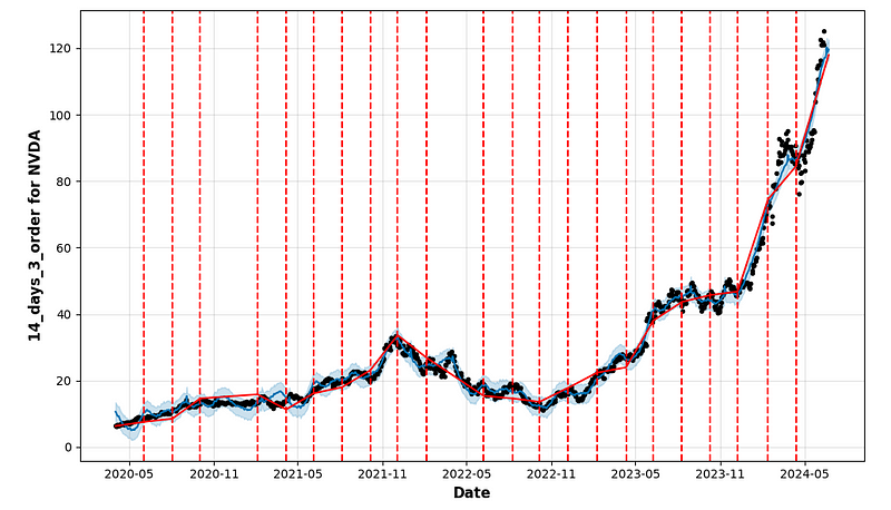
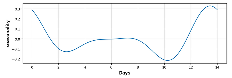
- period_days=14 & fourier_order_seasonality=12
- Performing cross-validation QC
res1=result['ypred']
print(res1[1])

1056    116.936342
1057    116.850275
1058    116.233301
1059    116.709060
1060    117.953234
1061    119.812505
1062    118.262082
1063    118.641367
1064    118.779563
1065    118.254753
Name: yhat, dtype: float64

print(valid_ts)

       ds           y
1056 2024-06-13  129.610001
1057 2024-06-14  131.880005
1058 2024-06-17  130.979996
1059 2024-06-18  135.580002
1060 2024-06-20  130.779999
1061 2024-06-21  126.570000
1062 2024-06-24  118.110001
1063 2024-06-25  126.089996
1064 2024-06-26  126.400002
1065 2024-06-27  123.989998

n=5
valid_ts['y'].plot(label='Validation')
res1[n].plot(label='Forecast')
plt.legend()
plt.xlabel('Time Sample')
plt.ylabel('Price')
plt.grid()

y_true=valid_ts['y']
y_pred=res1[5]
resr2 = calc_metrics('r2_score', y_true, y_pred)
resrmse = calc_metrics('rmse', y_true, y_pred)      # in coins
resmape = 100*calc_metrics('mape', y_true, y_pred)  # in %
print(resr2)
print(resrmse)
print(resmape)

-4.654220698172283
10.99633729407076
7.488504106783908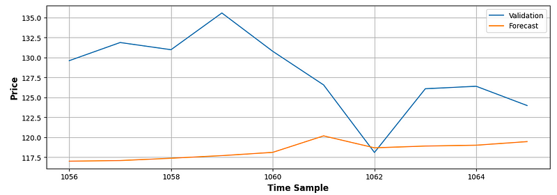
Auto-ARIMA Model Fitting
- This section is a demonstration on how to leverage Auto ARIMA functionality [1,5] using the pmdarima package to forecast the future NVDA stock price. The auto-ARIMA process seeks to identify the most optimal parameters for an ARIMA model, settling on a single fitted ARIMA model.
- Fetching and splitting the dataset
#ARIMA
# Get datasets
if is_ARIMA:
    train_ts, valid_ts, test_ts, train_valid_ts = get_train_valid_test_ts(df2.copy(), forecasting_days, target='Close')

Origin dataset has 1076 rows and 2 features
Get training dataset with 1056 rows
Get validation dataset with 10 rows
Get test dataset with 10 rows- Calculating and plotting ACF/PACF for the original time series and first-, second-order time differences
if is_ARIMA:
    # ACF and PACF
    lag_num = 100
    acf_pacf_draw(train_ts['y'], lag_num, True, True, 'Original Series')
    acf_pacf_draw(train_ts['y'].diff().dropna(), lag_num, True, True, '1st Order Differencing')
    acf_pacf_draw(train_ts['y'].diff().diff().dropna(), lag_num, True, True, '2nd Order Differencing')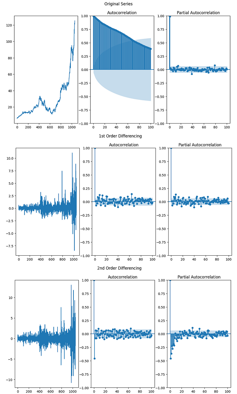
- Implementing ARIMA model fitting and Auto-ARIMA HPO
def arima_fit(df, col, order=(1,1,1)):
    # ARIMA model fitting for series df[col]

    model = sm.tsa.arima.ARIMA(df[col].values.squeeze(), order=order)
    model = model.fit()
    return model

def get_residual_errors(model):
    # Calculation and drawing the plot residual errors for ARIMA model
    residuals = pd.DataFrame(model.resid)
    fig, ax = plt.subplots(1,2, figsize=(12,6))
    residuals.plot(title="Residuals", ax=ax[0])
    residuals.plot(kind='kde', title='Density', ax=ax[1])
    plt.show()

def arima_forecasting(result, model, params, name_model, df, type_data):
    # Data df (validation or test) forecasting on the num days by the model
    # with params and save metrics to result

    ypred = model.forecast(steps=len(df))

    n = len(result)
    result.loc[n,'name_model'] = name_model
    result.loc[n,'type_data'] = type_data
    result.at[n,'params'] = params
    result.at[n,'ypred'] = ypred
    #result = result_add_metrics(result, n, df['y'], y_pred)

    return result

if is_ARIMA:
    # Automatic tuning of the ARIMA model
    model_auto = pm.auto_arima(train_ts['y'].values,
                               start_p=4,        # start p
                               start_q=4,        # start q
                               test='adf',       # use adftest to find optimal 'd'
                               max_p=5, max_q=5, # maximum p and q
                               m=1,              # frequency of series (1 - No Seasonality)
                               d=None,           # let model determine 'd'
                               seasonal=False,   # No Seasonality
                               start_P=0,
                               D=0,
                               start_Q=0,
                               trace=True,
                               error_action='ignore',
                               suppress_warnings=False,
                               stepwise=True     # use the stepwise algorithm outlined in Hyndman and Khandakar (2008)
                                                 # to identify the optimal model parameters.
                                                 # The stepwise algorithm can be significantly faster than fitting all
                                                 # hyper-parameter combinations and is less likely to over-fit the model
                              )

    print(model_auto.summary())

Performing stepwise search to minimize aic
 ARIMA(4,1,4)(0,0,0)[0] intercept   : AIC=inf, Time=1.19 sec
 ARIMA(0,1,0)(0,0,0)[0] intercept   : AIC=3278.225, Time=0.01 sec
 ARIMA(1,1,0)(0,0,0)[0] intercept   : AIC=3280.157, Time=0.04 sec
 ARIMA(0,1,1)(0,0,0)[0] intercept   : AIC=3280.146, Time=0.04 sec
 ARIMA(0,1,0)(0,0,0)[0]             : AIC=3286.435, Time=0.01 sec
 ARIMA(1,1,1)(0,0,0)[0] intercept   : AIC=3274.481, Time=0.25 sec
 ARIMA(2,1,1)(0,0,0)[0] intercept   : AIC=3276.898, Time=0.17 sec
 ARIMA(1,1,2)(0,0,0)[0] intercept   : AIC=3276.272, Time=0.30 sec
 ARIMA(0,1,2)(0,0,0)[0] intercept   : AIC=3276.936, Time=0.06 sec
 ARIMA(2,1,0)(0,0,0)[0] intercept   : AIC=3277.302, Time=0.05 sec
 ARIMA(2,1,2)(0,0,0)[0] intercept   : AIC=3277.648, Time=0.34 sec
 ARIMA(1,1,1)(0,0,0)[0]             : AIC=3282.470, Time=0.14 sec

Best model:  ARIMA(1,1,1)(0,0,0)[0] intercept
Total fit time: 2.629 seconds
                               SARIMAX Results
==============================================================================
Dep. Variable:                      y   No. Observations:                 1056
Model:               SARIMAX(1, 1, 1)   Log Likelihood               -1633.240
Date:                Wed, 17 Jul 2024   AIC                           3274.481
Time:                        14:06:03   BIC                           3294.326
Sample:                             0   HQIC                          3282.003
                               - 1056
Covariance Type:                  opg
==============================================================================
                 coef    std err          z      P>|z|      [0.025      0.975]
------------------------------------------------------------------------------
intercept      0.2192      0.076      2.876      0.004       0.070       0.369
ar.L1         -0.9472      0.020    -46.224      0.000      -0.987      -0.907
ma.L1          0.9748      0.016     59.838      0.000       0.943       1.007
sigma2         1.2946      0.020     64.815      0.000       1.255       1.334
===================================================================================
Ljung-Box (L1) (Q):                   0.16   Jarque-Bera (JB):             16930.67
Prob(Q):                              0.69   Prob(JB):                         0.00
Heteroskedasticity (H):              23.15   Skew:                             1.79
Prob(H) (two-sided):                  0.00   Kurtosis:                        22.30
===================================================================================- Getting orders of the best ARIMA model
if is_ARIMA:
    # Get orders of the best model from AutoARIMA
    arima_orders_best = list(model_auto.get_params().get('order'))
    print(f"Optimal parameters are {arima_orders_best}")
    model_auto = arima_fit(train_ts, 'y', order=(arima_orders_best[0],arima_orders_best[1],arima_orders_best[2]))

Optimal parameters are [1, 1, 1]- Plotting the Auto-ARIMA diagnostics summary
if is_ARIMA:
    # Best model from AutoARIMA
    fig = model_auto.plot_diagnostics(figsize=(12,10))
    plt.show()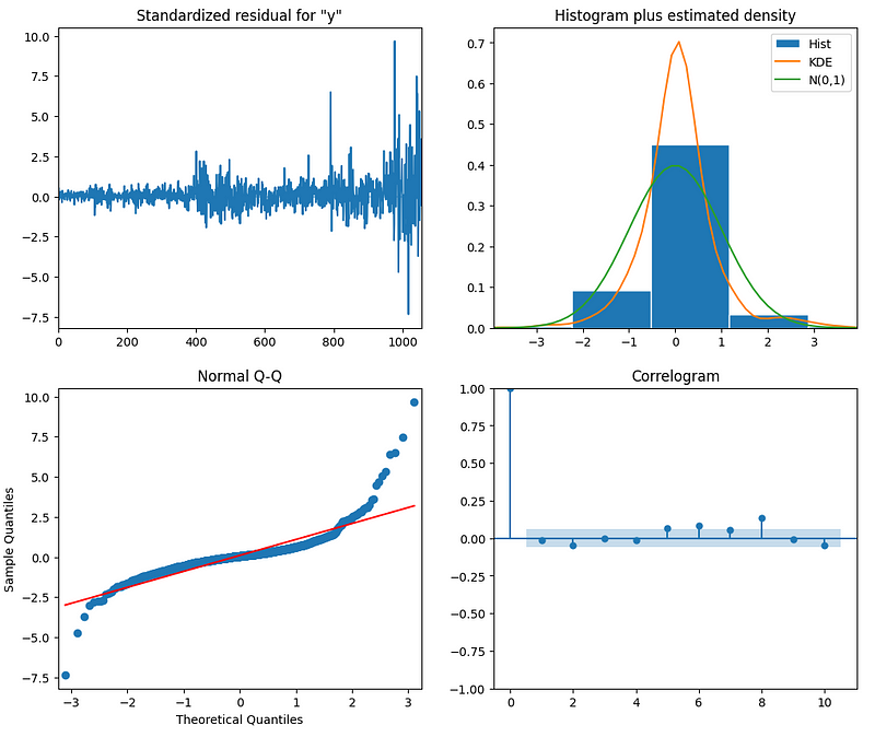
- Printing the final validation result
if is_ARIMA:
    # Valid forecasting and save result
    result = arima_forecasting(result, model_auto, arima_orders_best, 'ARIMA_auto', valid_ts, 'valid')

y_true=valid_ts['y']
y_pred=res1[0]
resr2 = calc_metrics('r2_score', y_true, y_pred)
resrmse = calc_metrics('rmse', y_true, y_pred)      # in coins
resmape = 100*calc_metrics('mape', y_true, y_pred)  # in %
print(resr2)
print(resrmse)
print(resmape)

-0.3756885596041244
5.424025684842693
3.472035737786662
SciKit-Learn Supervised ML Regression & HPO
- Let’s train/test the popular supervised ML regression models and optimize their hyperparameters available in SciKit-Learn [1,4].
- Hyperparameters are parameters that are not directly learnt within estimators. In Scikit-Learn they are passed as arguments to the constructor of the estimator classes [4].
- Fetching and splitting the input dataset
if is_other_ML:
    df2 = get_target_mf(df2, forecasting_days, col='Close')
    train_mf, ytrain_mf, valid_mf, yvalid_mf, test_mf, ytest_mf, train_valid_mf, y_train_valid_mf, starting_point = \
                                    get_train_valid_test_mf(df2.copy(), forecasting_days, target='target')

Origin dataset has 242 rows and 60 features
Get training dataset with 222 rows
Get validation dataset with 10 rows
Get test dataset with 10 rows- Defining the 8 supervised ML models with search hyperparameters
if is_other_ML:
    # Set parameters of models
    models = pd.DataFrame(columns = ['name', 'model', 'param_grid'])

    # Linear Regression
    n = len(models)
    models.loc[n, 'name'] = 'Linear Regression'
    models.at[n, 'model'] = LinearRegression()
    models.at[n, 'param_grid'] = {'fit_intercept' : [True, False]}


    # KNeighbors Regressor
    n = len(models)
    models.loc[n, 'name'] = 'KNeighbors Regressor'
    models.at[n, 'model'] = KNeighborsRegressor()
    models.at[n, 'param_grid'] = {'n_neighbors': [3, 5, 10, 20, 30],
                                  'leaf_size': [10, 20, 30]
                                 }

    # Support Vector Machines
    n = len(models)
    models.loc[n, 'name'] = 'Support Vector Machines'
    models.at[n, 'model'] = SVR()
    models.at[n, 'param_grid'] = {'kernel': ['linear', 'poly', 'rbf', 'sigmoid'],
                                  'C': np.linspace(1, 15, 15),
                                  'tol': [1e-3, 1e-4]
                                 }

    # Linear SVC
    n = len(models)
    models.loc[n, 'name'] = 'Linear SVR'
    models.at[n, 'model'] = LinearSVR()
    models.at[n, 'param_grid'] = {'C': np.linspace(1, 15, 15)}


    # Random Forest Classifier
    n = len(models)
    models.loc[n, 'name'] = 'Random Forest Regressor'
    models.at[n, 'model'] = RandomForestRegressor()
    models.at[n, 'param_grid'] = {'n_estimators': [40, 50, 60, 80],
                                  'min_samples_split': [30, 40, 50, 60],
                                  'min_samples_leaf': [10, 12, 15, 20, 50],
                                  'max_features': [100],
                                  'max_depth': [3, 4, 5, 6]
                                 }

    # Bagging Classifier
    n = len(models)
    models.loc[n, 'name'] = 'Bagging Regressor'
    models.at[n, 'model'] = BaggingRegressor()
    models.at[n, 'param_grid'] = {'max_features': np.linspace(0.05, 0.8, 1),
                                  'n_estimators': [3, 4, 5, 6],
                                  'warm_start' : [False]
                                 }

    # XGB Classifier
    n = len(models)
    models.loc[n, 'name'] = 'XGB Regressor'
    models.at[n, 'model'] = xgb.XGBRegressor()
    models.at[n, 'param_grid'] = {'n_estimators': [50, 70, 90],
                                  'learning_rate': [0.01, 0.05, 0.1, 0.2],
                                  'max_depth': [3, 4, 5]
                                 }

    # MLP Classifier
    n = len(models)
    models.loc[n, 'name'] = 'MLP Regressor'
    models.at[n, 'model'] = MLPRegressor()
    models.at[n, 'param_grid'] = {'hidden_layer_sizes': [i for i in range(2,5)],
                                  'solver': ['lbfgs', 'sgd'],
                                  'learning_rate': ['adaptive'],
                                  'learning_rate_init': [0.001, 0.01],
                                  'max_iter': [1000]
                                 }
models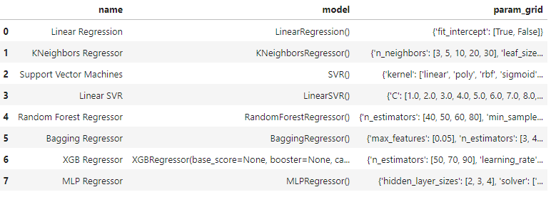
- Tuning the above ML models
def model_prediction(result, models, train_features, valid_features, train_labels, valid_labels):
    # Models training and data prediction for all models from DataFrame models
    # Saving results for validation dataset into dataframe result

    def calc_add_score(res, n, type_score, list_true, list_pred, feature_end):
        # Calculation score with type=type_score for list_true and list_pred
        # Adding score into res.loc[n,...]
        res.loc[i, type_score + feature_end] = calc_metrics(type_score, list_true, list_pred)
        return res

    # Results
    model_all = []

    for i in range(len(models)):
        # Training
        print(f"Tuning model '{models.loc[i, 'name']}'")
        model = GridSearchCV(models.at[i, 'model'], models.at[i, 'param_grid'])
        model.fit(train_features, train_labels)
        model_all.append(model)
        print(f"Best parameters: {model.best_params_}\n")

        # Prediction
        ypred = model.predict(valid_features)

        # Scoring and saving results into the main dataframe result
        n = len(result)
        result.loc[n,'name_model'] = f"{models.loc[i, 'name']}"
        result.loc[n,'type_data'] = "valid"
        result.at[n,'params'] = model.best_params_
        result.at[n,'ypred'] = ypred
        #result = result_add_metrics(result, n, valid_labels, valid_pred)

    return result, model_all

if is_other_ML:
    # Models tuning and the forecasting
    result, model_all = model_prediction(result, models, train_mf, valid_mf, ytrain_mf, yvalid_mf)

Tuning model 'Linear Regression'
Best parameters: {'fit_intercept': False}

Tuning model 'KNeighbors Regressor'
Best parameters: {'leaf_size': 10, 'n_neighbors': 30}

Tuning model 'Support Vector Machines'
Best parameters: {'C': 1.0, 'kernel': 'rbf', 'tol': 0.0001}

Tuning model 'Linear SVR'
Best parameters: {'C': 3.0}

Tuning model 'Random Forest Regressor'
Best parameters: {'max_depth': 6, 'max_features': 100, 'min_samples_leaf': 15, 'min_samples_split': 40, 'n_estimators': 40}

Tuning model 'Bagging Regressor'
Best parameters: {'max_features': 0.05, 'n_estimators': 6, 'warm_start': False}

Tuning model 'XGB Regressor'
Best parameters: {'learning_rate': 0.1, 'max_depth': 5, 'n_estimators': 70}

Tuning model 'MLP Regressor'
Best parameters: {'hidden_layer_sizes': 4, 'learning_rate': 'adaptive', 'learning_rate_init': 0.01, 'max_iter': 1000, 'solver': 's- Validating the optimized ML models and computing their r2_score, rmse, and mape [1]
def recovery_prediction(y, starting_point):
    # Recovering prediction of multi-factors model for shifted col_diff to col in the dataframe df
    # y has type np.array
    # starting_point is dictionary with start values for the recovering data
    # Returns y (np.array) with recovering data

    return np.insert(y, 0, starting_point).cumsum()[1:]

def result_recover_and_metrics(result, df_ts, type_data, start_points):
    # Recovering prediction: from shifted_Close_diff to Close
    # Calculation metrics for recovering ypred forecasting for all models in result
    # ypred real is from df_ts['y']
    # start points value for the recovering is from dictionary start_points
    # type_data = 'valid' or 'test'

    for i in range(len(result)):
        if (result.loc[i, 'type_data']==type_data) and (result.loc[i, 'mape'] is np.nan):
            ypred = result.loc[i, 'ypred']

            # Recovering ypred for multi-factors models
            if not (str(result.loc[i, 'type_model']) in ['Prophet', 'ARIMA']):
                # Multi-factors model
                # Get start points value for the recovering
                start_point_value = start_points['valid_start_point'] if type_data=='valid' else start_points['test_start_point']
                # Recovering prediction
                ypred = recovery_prediction(ypred, start_point_value)

            # Calculation metrics
            result = result_add_metrics(result, i, df_ts['y'], ypred)

    return result

# Dispay and save all results for validation dataset
if len(result) > 0:

    # Get type of each model
    result['type_model'] = result['name_model'].str.split('_').str[0]

    # Calculation metrics for recovering prediction ypred for validation dataset by all models
    result = result_recover_and_metrics(result, valid_ts, 'valid', starting_point)
    display(result[['name_model', 'type_data', 'r2_score', 'rmse', 'mape']].sort_values(by=['type_data', 'mape', 'rmse'], ascending=True))

    # Save results
    num_models = len(result[result['type_data']=='valid']['name_model'].unique().tolist())
    print(f"Number of models built - {num_models}")
    result.to_csv(f'result_of_{num_models}_models_for_forecasting_days_{forecasting_days}.csv')
else:
    print('There are no tuned models!')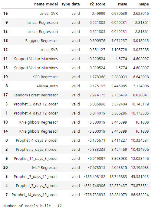
- Optimized ML model training and forecasting [1]
def get_model_opt(name_model, params):
# Model tuning for the name_model
print(name_model)
if name_model=='Linear Regression':
model = LinearRegression(**params)
elif name_model=='KNeighbors Regressor':
model = KNeighborsRegressor(**params)
elif name_model=='Support Vector Machines':
model = SVR(**params)
elif name_model=='Linear SVR':
model = LinearSVR(**params)
elif name_model=='Random Forest Regressor':
model = RandomForestRegressor(**params)
elif name_model=='Bagging Regressor':
model = BaggingRegressor(**params)
elif name_model=='MLP Regressor':
model = MLPRegressor(**params)
elif name_model=='XGB Regressor':
model = xgb.XGBRegressor(**params)
else: model = None
return model
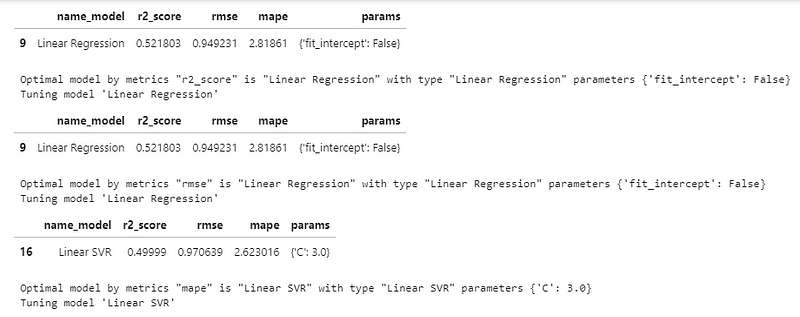
def get_params_optimal_model(result, main_metrics):
# Get parameters of the optimal model from dataframe result by main_metrics
# Set the data type to float (just in case)
result[main_metrics] = result[main_metrics].astype('float')
# Choose the optimal model
opt_result = result[result['type_data']=='valid'].reset_index(drop=True)
if main_metrics=='r2_score':
opt_model = opt_result.nlargest(1, main_metrics)
else:
# 'mape' or 'rmse'
opt_model = opt_result.nsmallest(1, main_metrics)
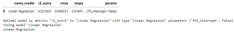
display(opt_model[['name_model', 'r2_score', 'rmse', 'mape', 'params']])
# Get parameters of the optimal model
opt_name_model = opt_model['name_model'].tolist()[0]
opt_type_model = opt_model['type_model'].tolist()[0]
opt_params_model = opt_model['params'].tolist()[0]
print(f'Optimal model by metrics "{main_metrics}" is "{opt_name_model}" with type "{opt_type_model}" parameters {opt_params_model}')
return opt_name_model, opt_type_model, opt_params_model
def model_training_forecasting(result, df, y, test, ytest,
name_model, type_model, params, type_test='1'):
# Model training for df and y
# Forecasting ypred
# type_model = 'Prophet' or "ARIMA" or 'Other ML'
# type_test = '1' (with find optimal parameters by GridSearchCV)
# type_test = '2' (with optimal parameters - without GridSearchCV)
# return params and metrics in the dataframe result
if type_model=='Prophet':
season_days_optimal = params[0]
fourier_order_seasonality_optimal = params[1]
model_opt = None
_, ypred = prophet_modeling(result,
cryptocurrency,
df,
test,
holidays_df,
season_days_optimal,
fourier_order_seasonality_optimal,
forecasting_days,
f'{type_model}_optimal',
'test')
elif type_model=='ARIMA':
season_days_optimal = params[0]
fourier_order_seasonality_optimal = params[1]
model_opt = None
# Training ARIMA optimal model for training+valid dataset
df['y'] = y
model_opt = arima_fit(df, 'y', order=(params[0],params[1],params[2]))
# Model diagnostics
fig = model_opt.plot_diagnostics(figsize=(12,10))
plt.show()
# Plot residual errors
get_residual_errors(model_opt)
# Test forecasting and save result
ypred = model_opt.forecast(steps=len(test))
else:
# Other ML model
# Training ML optimal model for training+valid dataset
print(f"Tuning model '{name_model}'")
models_opt_number = models[models['name']==name_model].index.tolist()[0]
#print(f"Model - {models.at[models_opt_number,'model']} with parameters {params}")
if type_test=='1':
model_opt = GridSearchCV(models.at[models_opt_number,'model'], models.at[models_opt_number,'param_grid'])
else:
# type_test=='2'
model_opt = get_model_opt(models.at[models_opt_number,'name'], params)
model_opt.fit(df, y)
# Forecasting
ypred = model_opt.predict(test)
# Scoring and saving results into the dataframe result
n = len(result)-1
result.loc[n,'name_model'] = f"{type_model}_optimal"
result.loc[n,'type_data'] = "test"
result.loc[n,'type_model'] = type_model
result.at[n,'params'] = params
result.at[n,'ypred'] = ypred
#result = result_add_metrics(result, n, ytest, ypred)
return result, model_opt, ypred
def get_optimal_model_and_forecasting(result, main_metrics, start_points):
# Choosion the optimal model from dataframe result by main_metrics
# Tuning optimal model for big dataset train+valid
# Test forecasting and drawing it
# Returns the optimal model and it's name
if len(result) > 0:
# Get parameters of the optimal model from dataframe result by main_metrics
opt_name_model, opt_type_model, opt_params_model = get_params_optimal_model(result,
main_metrics)
# Set datasets for the final tuning and testing by optimal model
if (opt_type_model=='Prophet') or (opt_type_model=='ARIMA'):
train_valid = train_valid_ts.copy()
y_train_valid = train_valid_ts['y'].copy()
test = test_ts.copy()
ytest = test_ts['y'].copy()
else:
# Multi-factors ML models
train_valid = train_valid_mf.copy()
y_train_valid = y_train_valid_mf.copy()
test = test_mf.copy()
ytest = ytest_mf.copy()
# Optimal model training for train+valid and test forecasting
result, model_opt, ypred = model_training_forecasting(result, train_valid, y_train_valid,
test, ytest,
opt_name_model, opt_type_model,
opt_params_model, '1')
# Calculation metrics for recovering prediction ypred for test dataset by the optimal model
result = result_recover_and_metrics(result, test_ts, 'test', start_points)
# Drawing plot for prediction for the test data
if not ((opt_type_model=='Prophet') or (opt_type_model=='ARIMA')):
# Recovery values "Close"
ytest_plot = recovery_prediction(ytest.values, start_points['test_start_point'])
ypred_plot = recovery_prediction(ypred, start_points['test_start_point'])
else:
ytest_plot = ytest.copy()
ypred_plot = ypred.copy()
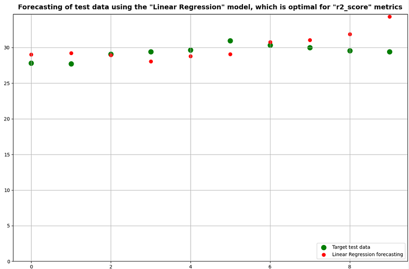
# Drawing
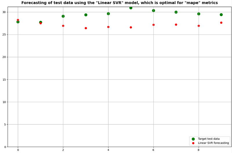
plt.figure(figsize=(12,8))
x = np.arange(len(ytest_plot))
plt.scatter(x, ytest_plot, label = "Target test data", color = 'g', s=100)
plt.scatter(x, ypred_plot, label = f"{opt_name_model} forecasting", color = 'r', s=50)
plt.title(f'Forecasting of test data using the "{opt_name_model}" model, which is optimal for "{main_metrics}" metrics')
plt.ylim(0)
plt.legend(loc='lower right')
plt.grid(True)
return opt_name_model
# Get the optimal model by different metrics
if len(result) > 0:
for valid_metrics in ['r2_score', 'rmse', 'mape']:
get_optimal_model_and_forecasting(result, valid_metrics, starting_point)
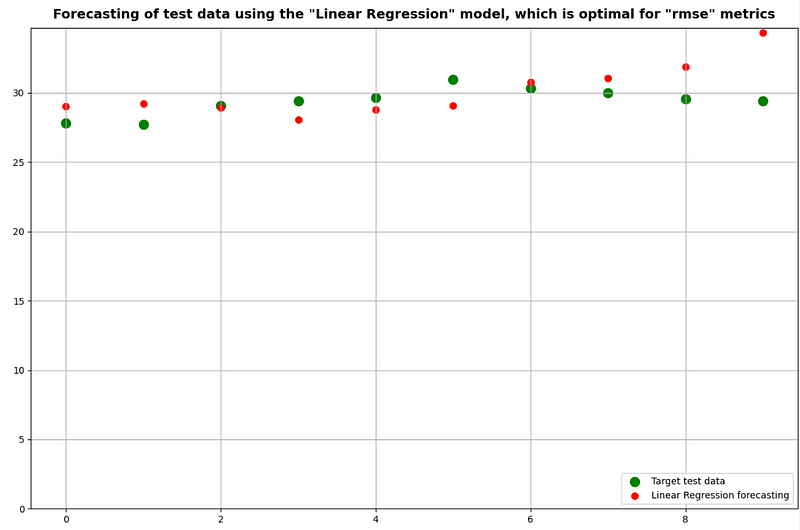
- Getting the best Linear Regression model
if is_other_ML:
    main_metrics = 'r2_score'
    if (len(result) > 0) and (len(models) > 0):
        result_nonTS = result[(result['type_model']!='Prophet') & (result['type_model']!='ARIMA')].reset_index(drop=True)
        opt_name_model2, opt_type_model2, opt_params_model2 = get_params_optimal_model(result_nonTS,
                                                                                main_metrics)

        result, model_opt, ypred = model_training_forecasting(result,
                                                              train_valid_mf,
                                                              y_train_valid_mf,
                                                              test_mf,
                                                              ytest_mf,
                                                              opt_name_model2,
                                                              opt_type_model2,
                                                              opt_params_model2,
                                                              '2')
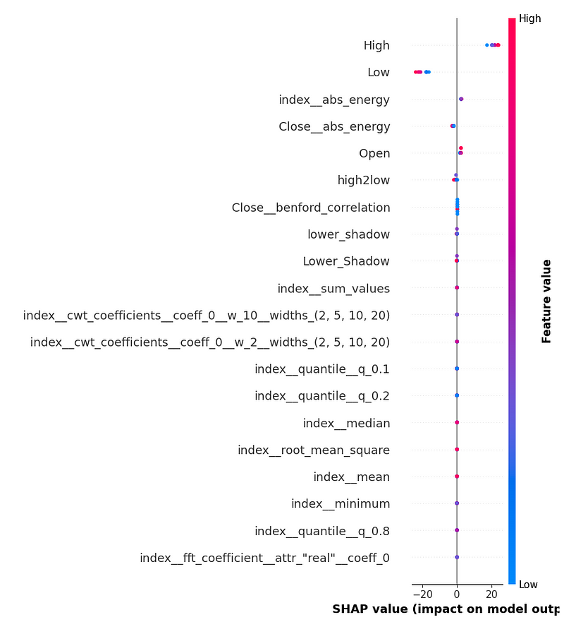
SHAP Feature Dominance Analysis
- Let’s use the SHAP package to calculate feature importance [1, 6]. The most common way of understanding ML models is to examine the coefficients learned for each feature.
- Plotting the feature importance diagrams with SHAP [1]
# All features names
if is_other_ML:
    coeff = pd.DataFrame(train_valid_mf.columns)
    coeff.columns = ['feature']

def add_fi_coeff(coeff, col, list_new_fi_coeff=None, df_new_fi_coeff=None):
    # Adds new importance of features as feature col
    # from list list_new_fi_coeff or dataframe df_new_fi_coeff
    # to the resulting dataframe coeff with feature names
    # Missed importance values are replaced by zero

    if list_new_fi_coeff is not None:
        df_new_fi_coeff = coeff[['feature']].copy()
        df_new_fi_coeff["score"] = pd.Series(list_new_fi_coeff)

    if df_new_fi_coeff is not None:
        # Rename df_new_fi_coeff
        df_new_fi_coeff.columns = ['feature', 'score']   # to the plot drawing
        df_new_fi_coeff[col] = df_new_fi_coeff['score']  # to the merging and saving

        # Merging dataframes - coeff of all features with new_fi_coeff
        coeff = coeff.merge(df_new_fi_coeff[['feature', col]], on='feature', how='left').fillna(0)

        is_score = True
    else:
        print(f'Data is absent fol {col}')
        is_score = False
        coeff = None

    return coeff, df_new_fi_coeff, is_score

# Feature importance diagram with SHAP
if is_other_ML:
    if (len(result) > 0) and (len(models) > 0):
        print('Feature importance diagram with SHAP:')
        try:
            # Trees
            explainer = shap.TreeExplainer(model_opt)
            shap_values = explainer.shap_values(test_mf)
            shap.summary_plot(shap_values, test_mf, plot_type="bar", feature_names=coeff['feature'].tolist())
            shap.summary_plot(shap_values, test_mf)

            # Save permutation feature importance values
            coeff, _, is_SHAP_successfully = add_fi_coeff(coeff, 'shap_fi_score', shap_values)
        except:
            try:
                # Other types of models
                explainer = shap.KernelExplainer(model_opt.predict, train_valid_mf)
                shap_values = explainer.shap_values(test_mf)

                # Plot drawing
                shap.summary_plot(shap_values, test_mf, plot_type="bar", feature_names=coeff['feature'].tolist())
                shap.summary_plot(shap_values, test_mf)

                # Get feature importance values from shap_values format
                # Thanks to https://stackoverflow.com/a/69523421/12301574
                shap_values_all = pd.DataFrame(shap_values, columns = test_mf.columns)
                vals = np.abs(shap_values_all.values).mean(0)
                shap_importance = pd.DataFrame(list(zip(test_mf.columns, vals)),
                                                  columns=['feature','score'])

                # Saving feature importance values
                coeff, _, is_SHAP_successfully = add_fi_coeff(coeff, 'shap_fi_score', None, shap_importance)

            except:
                is_SHAP_successfully = False

        if not is_SHAP_successfully:
            print('Feature importance diagram for this optimal model is not supported in SHAP')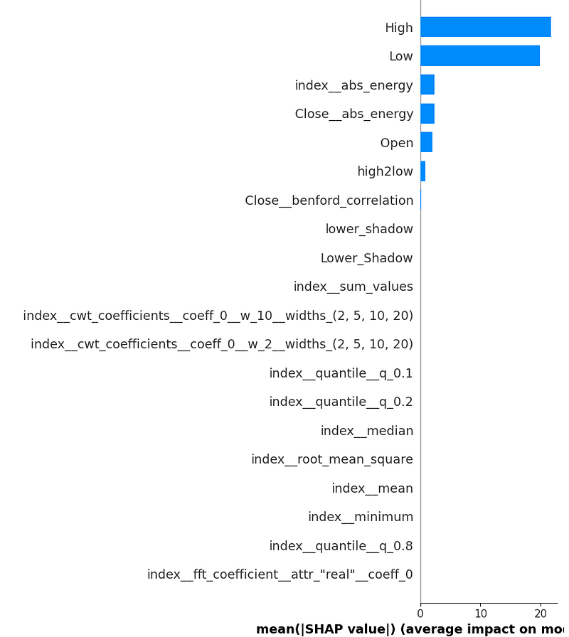
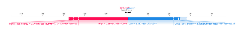
- Creating the Feature importance diagram as the Force plot with SHAP
LSTM Prediction & Validation QC
- LSTMs are an improved version of recurrent neural networks (RNNs).
- Here, we demonstrate how the LSTM algorithm [7] can be used to predict NVDA stock prices by training on historical data.
- Importing the relevant Python libraries and reading the stock data
import pandas as pd
import numpy as np

import matplotlib.pyplot as plt
import seaborn as sns
sns.set_style('whitegrid')
plt.style.use("fivethirtyeight")
%matplotlib inline

# For reading stock data from yahoo
from pandas_datareader.data import DataReader

# For time stamps
from datetime import datetime
from math import sqrt
from math import sqrt
from sklearn.metrics import mean_squared_error
from sklearn.preprocessing import MinMaxScaler

#ignore the warnings
import warnings
warnings.filterwarnings('ignore')

from keras.models import Sequential
from keras.layers import Dense, LSTM
import tensorflow as tf

#!pip install keras
#!pip install tensorflow

def plot_close_val(data_frame, column, stock):
    plt.figure(figsize=(12,6))
    plt.title(column + ' Price History for ' + stock )
    plt.plot(data_frame[column])
    plt.xlabel('Date', fontsize=18)
    plt.ylabel(column + ' Price USD ($) for ' + stock, fontsize=18)
    plt.show()

#Test the function
plot_close_val(df, 'Close', 'NVDA')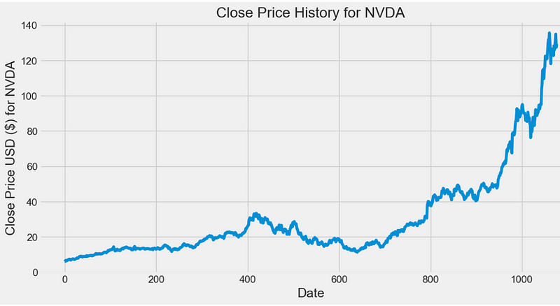
- Preparing the input data for LSTM model training
def build_training_dataset(input_ds):
    # Create a new dataframe with only the 'Close column
    input_ds.reset_index()
    data = input_ds.filter(items=['Close'])
    # Convert the dataframe to a numpy array
    dataset = data.values
    # Get the number of rows to train the model on
    training_data_len = int(np.ceil( len(dataset) * .90 ))
    return data, dataset, training_data_len

#Test the function
training_data_df, training_dataset_np, training_data_len = build_training_dataset(df)
dataset=training_dataset_np
data=training_data_df

# Scale the data
from sklearn.preprocessing import MinMaxScaler
def scale_the_data(dataset):
    scaler = MinMaxScaler(feature_range=(0,1))
    scaled_data = scaler.fit_transform(dataset)
    return scaler, scaled_data

#Test the function
scaler, scaled_data = scale_the_data(training_dataset_np)

# Create the training data set
# Create the scaled training data set
def split_train_dataset(training_data_len):
    train_data = scaled_data[0:int(training_data_len), :]
    # Split the data into x_train and y_train data sets
    x_train = []
    y_train = []
    for i in range(60, len(train_data)):
        x_train.append(train_data[i-60:i, 0])
        y_train.append(train_data[i, 0])
        if i<= 61:
            #print(x_train)
            #print(y_train)
            print('.')

    # Convert the x_train and y_train to numpy arrays
    x_train, y_train = np.array(x_train), np.array(y_train)

    # Reshape the data
    x_train = np.reshape(x_train, (x_train.shape[0], x_train.shape[1], 1))
    # x_train.shape
    return x_train, y_train

#Test the function
x_train,y_train = split_train_dataset(training_data_len)- Building the LSTM model
def build_lstm_model(x_train,y_train):
    # Build the LSTM model
    model = Sequential()
    model.add(LSTM(128, return_sequences=True, input_shape= (x_train.shape[1], 1)))
    model.add(LSTM(64, return_sequences=False))
    model.add(Dense(25))
    model.add(Dense(1))

    # Compile the model
    model.compile(optimizer='adam', loss='mean_squared_error')
    #model.compile(optimizer='lion', loss='mean_squared_error')
    #model.compile(optimizer='adamw', loss='mean_squared_error')
    # Train the model
    model.fit(x_train, y_train, batch_size=2, epochs=10)
    return model

#Test the function
lstm_model = build_lstm_model(x_train,y_train)
- Making test data predictions with TEST_DATA_LENGTH = 100
def create_testing_data_set(model, scaler, training_data_len,test_data_len):
    # Create the testing data set
    #
    test_data = scaled_data[training_data_len - test_data_len: , :]
    # Create the data sets x_test and y_test
    x_test = []
    y_test = dataset[training_data_len:, :]
    for i in range(test_data_len, len(test_data)):
        x_test.append(test_data[i-test_data_len:i, 0])

    # Convert the data to a numpy array
    x_test = np.array(x_test)

    # Reshape the data
    x_test = np.reshape(x_test, (x_test.shape[0], x_test.shape[1], 1 ))

    # Get the models predicted price values
    predictions = model.predict(x_test)
    predictions = scaler.inverse_transform(predictions)

    # Get the root mean squared error (RMSE)
    rmse = np.sqrt(np.mean(((predictions - y_test) ** 2)))
    print(rmse)
    return (x_test, y_test, predictions, rmse)

#Test the function
TEST_DATA_LENGTH = 100
x_test,y_test, predictions, rmse = create_testing_data_set(lstm_model,scaler,training_data_len, TEST_DATA_LENGTH)

4.706425009397595- Comparing test data vs LSTM predictions
plt.figure(figsize=(12,6))
plt.plot(y_test,label='Test')
plt.plot(predictions,label='Prediction')
plt.xlabel('Forecast Day No')
plt.ylabel('Price')
plt.legend()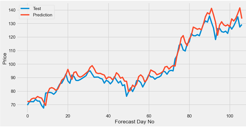
- Comparing validation data vs LSTM predictions
def plot_predictions(stock, data,training_data_len):
    #Plot the data
    train = data[:training_data_len]
    valid = data[training_data_len:]
    valid['Predictions'] = predictions
    # Visualize the data
    plt.figure(figsize=(14,6))
    title = stock + ' Model Forecast'
    ylabel = stock + ' Close Price USD ($)'
    plt.title(title)
    plt.xlabel('Date', fontsize=18)
    plt.ylabel(ylabel, fontsize=18)
    plt.plot(train['Close'])
    plt.plot(valid[['Close', 'Predictions']])
    plt.legend(['Training Data', 'Validated Data', 'Predicted Data'], loc='lower right')
    plt.show()
    return valid

#Test the function
valid = plot_predictions('NVDA',data,training_data_len)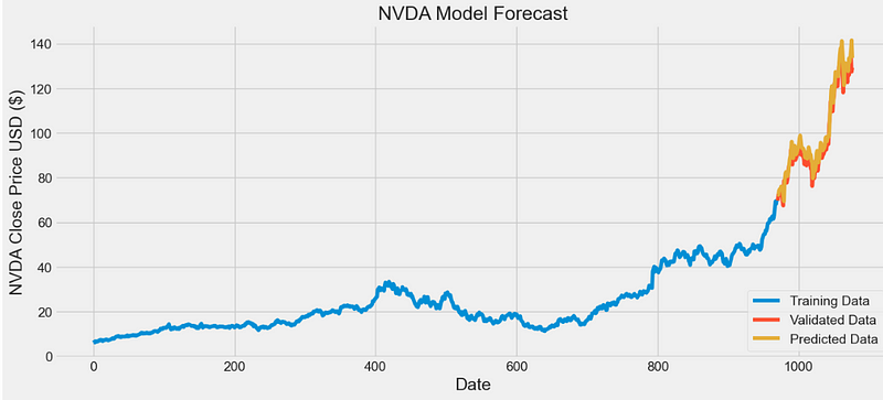
- Calculating the LSTM error metrics
from sklearn.metrics import r2_score
r2_score(y_test, predictions)

0.9375826947059053

from sklearn.metrics import root_mean_squared_error
root_mean_squared_error(y_test, predictions)

4.706425009397595


from sklearn.metrics import mean_absolute_error
mean_absolute_error(y_test, predictions)

3.7365759733681365

from sklearn.metrics import mean_absolute_percentage_error
mean_absolute_percentage_error(y_test, predictions)

0.03859417843438189

from sklearn.metrics import explained_variance_score
explained_variance_score(y_test, predictions)

0.9638450129795046- Plotting the LSTM model loss vs epochs for both train and test data
model = Sequential()
model.add(LSTM(128, return_sequences=True, input_shape= (x_train.shape[1], 1)))
model.add(LSTM(64, return_sequences=False))
model.add(Dense(25))
model.add(Dense(1))

    # Compile the model
model.compile(optimizer='adam', loss='mean_squared_error',metrics=['accuracy'])
    #model.compile(optimizer='lion', loss='mean_squared_error')
    #model.compile(optimizer='adamw', loss='mean_squared_error')
    # Train the model
history=model.fit(x_train, y_train, batch_size=2, epochs=10,validation_split=0.5)
# summarize history for loss
plt.plot(history.history['loss'])
plt.plot(history.history['val_loss'])
plt.title('model loss')
plt.ylabel('loss')
plt.xlabel('epoch')
plt.legend(['train', 'test'], loc='upper right')
plt.show()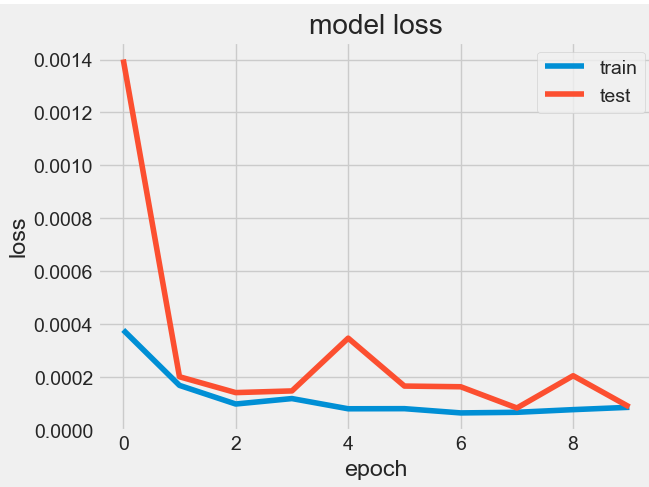
Conclusions
- In this article, we have applied the the concept of algorithmic trading to the NVIDIA Short-Term Stock Price Forecasting.
- We’ve walked through the following topics:
- Exploratory Data Analysis (EDA) of Input Stock Data
- Basic Linear Regression with Time-Step & Lag Features
- TSFRESH Feature Engineering [1]
- Multi-Seasonal FB Prophet Prediction & HPO
- Auto-ARIMA Model Fitting & SARIMAX QC Summary
- SciKit-Learn Supervised ML Regression & HPO
- SHAP Feature Dominance Analysis
- TF LSTM Keras Prediction & Validation QC
- We have shown that time series forecasting (predicting future values based on historical values) applies well to NVIDIA stock forecasting.
- Since stock prices prediction is essentially a regression problem, the R2-Score, RMSE, MAE, and MAPE have been our key model evaluation metrics.
- Using the LSTM algorithm [7] and the basic Linear Regression [2] of 10-day Lags, our results showed that the forecasting model has a high accuracy of >95% for most of the stock data used, demonstrating the appropriateness of the ML model and the test set data is used to evaluate the model’s performance.
- Our ongoing efforts focus on addressing the following challenges:
- Market Uncertainty: Financial markets can be highly unpredictable, making accurate predictions challenging.
- External Factors: Models may not account for sudden geopolitical events or economic shifts.
- Overfitting: Models may perform well on historical data but struggle with new, unforeseen patterns.
Acknowledgements
- The main code of this notebook was written or compiled from many notebooks by Kaggle Grandmaster, Dr. Eng. Sc., Prof. Vitalii Mokin.
References
- Crypto — BTC : Analysis & Forecasting
- Linear Regression With Time Series
- NVIDIA Stock Price Prediction
- SciKit-Learn Supervised Learning
- Forecasting Time Series with Auto-Arima
- Explaining individual predictions when features are dependent: More accurate approximations to Shapley values
- NASDAQ Stock Price Prediction using LSTM
Explore More
- An Integrated Quant Trading Analysis of US Big Techs using Quantstats, TA, PyPortfolioOpt, and FinanceToolkit
- NVDA Technical Analysis using 75 Simplified FinTA Indicators
- Backtesting Hull Moving Average (HMA) Algo-Trading: NVDA Price vs Volume Buy/Sell Signals & Expected Returns
- NVIDIA Returns-Drawdowns MVA & RNN Mean Reversal Trading
- NVIDIA Rolling Volatility: GARCH & XGBoost
- IQR-Based Log Price Volatility Ranking of Top 19 Blue Chips
- Returns-Volatility Domain K-Means Clustering and LSTM Anomaly Detection of S&P 500 Stocks
Contacts
Disclaimer
- The following disclaimer clarifies that the information provided in this article is for educational use only and should not be considered financial or investment advice.
- The information provided does not take into account your individual financial situation, objectives, or risk tolerance.
- Any investment decisions or actions you undertake are solely your responsibility.
- You should independently evaluate the suitability of any investment based on your financial objectives, risk tolerance, and investment timeframe.
- It is recommended to seek advice from a certified financial professional who can provide personalized guidance tailored to your specific needs.
- The tools, data, content, and information offered are impersonal and not customized to meet the investment needs of any individual. As such, the tools, data, content, and information are provided solely for informational and educational purposes only.


