Backtesting Hull Moving Average (HMA) Algo-Trading: NVDA Price vs Volume Buy/Sell Signals & Expected Returns

The objective of this post is to effectively backtest two Nvidia (NASDAQ: NVDA) algo-trading strategies based on the Hull Moving Average (HMA) trading indicator.
According to Zacks, NVDA is a top growth stock for the long-term. NVDA is a #2 (Buy) on the Zacks Rank, with a VGM Score of B. NVDA has a Growth Style Score of A, forecasting year-over-year earnings growth of 84.7% for the current fiscal year. With a solid Zacks Rank and top-tier Growth and VGM Style Scores, NVDA should be on investors’ short list.
Our current goal is to compare expected returns generated by HMA NVDA historical price vs volume crossover signals, being referred to as Strategies A and B, respectively.
While many traders focus solely on trading strategies that utilize price data only (Strategy A), we will delve into the importance of volume analysis and explore how Strategy B can provide insights into potential market trends and strength.

Price-Volume HMA Crossover Strategies

Conventionally, the HMA crossover strategy involves using two different HMA timeframes, a shorter period and a longer period, to generate trading signals when they cross each other.
The key idea is to generate buy and sell signals based on the interaction between the two HMA lines. As with other moving average indicators, when the price/volume crosses above the HMA line from below, it is considered a buy signal. Conversely, when the price/volume crosses below the HMA line from above, it is a sell signal.
Generally, the HMA strategy reduces noise in the data and provides clearer buy or sell signals when used alongside other technical indicators like oscillators or trend lines.
Unlike other moving averages that rely solely on closing prices, Strategy A takes into account high and low prices as well. This additional information helps smooth out volatility and provides a more comprehensive view of market dynamics.
In the proposed technical analysis, Strategies A and B are combined specifically to support investors that incorporate price-volume relationships into their trading decisions.

Let’s explore nuts & bolts of the HMA algo-trading strategies, covering everything from their implementation in Python to backtesting NVDA HMA price vs volume entry/exit positions and expected cumulative returns of Strategies A and B.

Downloading Stock Data

Importing libraries and reading the NVDA historical stock data 2022–2024

import datetime as dt
import pandas as pd 
import numpy as np
import matplotlib.pyplot as plt 

plt.style.use('fivethirtyeight')
plt.rcParams['figure.figsize'] = (20,10)

def download_stock_data(ticker,timestamp_start,timestamp_end):
    url=f"https://query1.finance.yahoo.com/v7/finance/download/{ticker}?period1={timestamp_start}&period2={timestamp_end}&interval\
=1d&events=history&includeAdjustedClose=true"
    df = pd.read_csv(url)
    return df

datetime_start=dt.datetime(2022, 1, 1, 7, 35, 51)
datetime_end=dt.datetime.today()

# Convert to timestamp:
timestamp_start=int(datetime_start.timestamp()) 
timestamp_end=int(datetime_end.timestamp()) 

ticker='NVDA'

df = download_stock_data(ticker,timestamp_start,timestamp_end)
df = df.set_index('Date')
df.tail()
           Open       High       Low        Close     Adj Close   Volume
Date      
2024-05-13 904.780029 909.979980 885.289978 903.989990 903.989990 28968000
2024-05-14 895.989990 916.510010 889.340027 913.559998 913.559998 29650700
2024-05-15 924.719971 948.619995 915.989990 946.299988 946.299988 41773500
2024-05-16 949.099976 958.190002 941.030029 943.590027 943.590027 32395200
2024-05-17 943.690002 947.400024 918.059998 924.789978 924.789978 34651900

Plotting SMA20 vs HMA20

Calculating and plotting 20-day HMA vs SMA for Adj Close price

def hma(period):
 wma_1 = df['Adj Close'].rolling(period//2).apply(lambda x: \
 np.sum(x * np.arange(1, period//2+1)) / np.sum(np.arange(1, period//2+1)), raw=True)
 wma_2 = df['Adj Close'].rolling(period).apply(lambda x: \
 np.sum(x * np.arange(1, period+1)) / np.sum(np.arange(1, period+1)), raw=True)
 diff = 2 * wma_1 - wma_2
 hma = diff.rolling(int(np.sqrt(period))).mean()
 return hma
period = 20
df['hma'] = hma(period)
df['SMA20'] = df['Adj Close'].rolling(period).mean()
figsize = (10,6)
df[['Adj Close','hma','SMA20']].plot(figsize=figsize)
plt.title('Hull Moving Average {0} days'.format(period))
plt.show()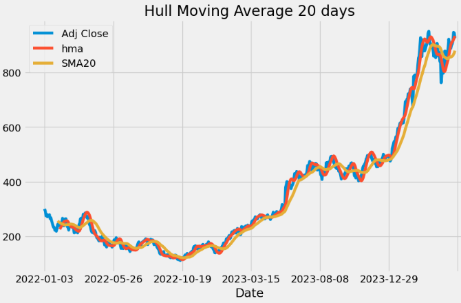

Plotting HMA Short/Long Lines

Calculating and plotting short (20-day) and long (30-day) HMA lines

df['hma_short']=hma(20)
df['hma_long']=hma(30)
figsize = (12,6)
df[['Adj Close','hma_short','hma_long']].plot(figsize=figsize)
plt.title('Hull Moving Average')
plt.show()

Short (20-day) and long (30-day) HMA lines

Comparing HMA Volume vs Period

Invoking the volume to calculate the weighted average

def hma_volume(period):
 wma_1 = df['nominal'].rolling(period//2).sum()/df['Volume'].rolling(period//2).sum()
 wma_2 = df['nominal'].rolling(period).sum()/df['Volume'].rolling(period).sum()
 diff = 2 * wma_1 - wma_2
 hma = diff.rolling(int(np.sqrt(period))).mean()
 return hma
df['nominal'] = df['Adj Close'] * df['Volume']
period = 20
df['hma_volume']=hma_volume(period)
figsize=(12,8)
fig, (ax0,ax1) = plt.subplots(nrows=2, sharex=True, subplot_kw=dict(frameon=True),figsize=figsize) 
df[['Adj Close','hma_volume','hma']].plot(ax=ax0)
ax0.set_title('HMA Volume vs HMA period')
df[['Volume']].plot(ax=ax1)
ax1.set_title('Hull Moving Average')
plt.show()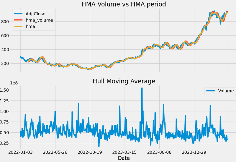

Backtesting Strategy A

Calculating trading signals and cumulative returns (CR) of Strategy A

#SIGNAL
df['hma_short']=hma(20)
df['hma_long']=hma(30)
df['signal'] = np.where(df['hma_short'] > df['hma_long'],1,-1)

#RETURN
df['signal_shifted']=df['signal'].shift()

## Calculate the returns on the days we trigger a signal
df['returns'] = df['Adj Close'].pct_change()

## Calculate the strategy returns
df['strategy_returns'] = df['signal_shifted'] * df['returns']

## Calculate the cumulative returns
df1=df.dropna()
df1['cumulative_returns'] = (1 + df1['strategy_returns']).cumprod()

#PLOT
figsize=(12,8)
fig, (ax0,ax1) = plt.subplots(nrows=2, sharex=True, subplot_kw=dict(frameon=True),figsize=figsize) 
df[['Adj Close','hma_long','hma_short']].plot(ax=ax0)
ax0.set_title("HMA: Short vs Long")

df[['signal']].plot(ax=ax1,style='-.',alpha=0.4)
ax1.legend()
ax1.set_title("HMA - Signals")
plt.show()

df1['cumulative_returns'].plot(figsize=(10,4))
plt.title("Cumulative Return")
plt.show()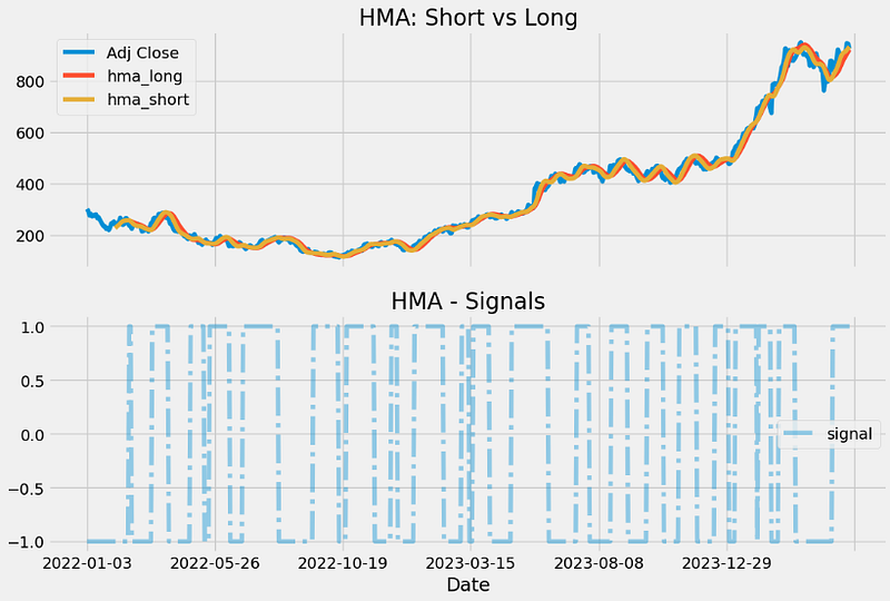

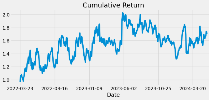
HMA Price Short vs Long Cumulative Return

Printing the latest value of CR

df1['cumulative_returns'].tail()[-1]

1.7016343263088096

Backtesting Strategy B

Calculating trading signals and cumulative returns (CR) of Strategy B

#SIGNAL
df['hma_volume_short']=hma_volume(20)
df['hma_volume_long']=hma_volume(30)
df['signal'] = np.where(df['hma_volume_short'] > df['hma_volume_long'],1,-1)

#RETURN
df['returns'] = df['Adj Close'].pct_change()

## Calculate the strategy returns
df['strategy_returns'] = df['signal'].shift() * df['returns']

## Calculate the cumulative returns
df2=df.dropna()
df2['cumulative_returns_volume'] = (1 + df2['strategy_returns']).cumprod()

# PLOT
figsize=(12,8)
fig, (ax0,ax1) = plt.subplots(nrows=2, sharex=True, subplot_kw=dict(frameon=True),figsize=figsize) 
df[['Adj Close','hma_volume_short','hma_volume_long']].plot(ax=ax0)
df[['signal']].plot(ax=ax1,style='-.',alpha=0.4)
ax0.set_title("HMA - Volume: Short vs Long")
ax1.legend()
plt.title("HMA - Signals")
plt.show()

figs = (10,4)
df2['cumulative_returns_volume'].plot(figsize = figs)
plt.title("Cumulative Return")
plt.show()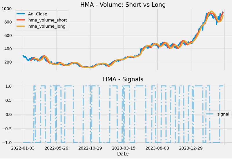

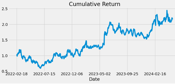
HMA Volume Short vs Long Trading Signals

HMA Volume Short vs Long Cumulative Return

Printing the latest value of CR

df2['cumulative_returns_volume'].tail()[-1]

2.1535115868707386

Trading Signals of Strategies A and B

Comparing trading signals of Strategies A and B

df['signal'] = np.where(df['hma_short'] > df['hma_long'],1,-1)
df['signal_volume'] = np.where(df['hma_volume_short'] > df['hma_volume_long'],1,-1)
figsize=(12,8)
df[['signal','signal_volume']].plot(figsize=figsize)
plt.show()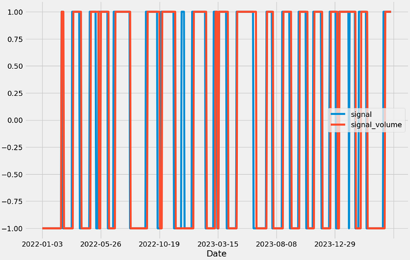

Backtesting Buy & Hold Strategy

Calculating expected returns of the NVDA Buy/Hold passive strategy

# Selecting libraries
import yfinance as yf
import pandas as pd
import numpy as np

benchmark='NVDA'
def get_benchmark(start_date, investment_value):
    spy=yf.download(benchmark, start=start_date)['Adj Close']
    benchmark1 = pd.DataFrame(np.diff(spy)).rename(columns = {0:'benchmark_returns'})
    
    investment_value = investment_value
    number_of_stocks = floor(investment_value/spy[0])
    benchmark_investment_ret = []
    
    for i in range(len(benchmark1['benchmark_returns'])):
        returns = number_of_stocks*benchmark1['benchmark_returns'][i]
        benchmark_investment_ret.append(returns)

    benchmark_investment_ret_df = pd.DataFrame(benchmark_investment_ret).rename(columns = {0:'investment_returns'})
    return benchmark_investment_ret_df

benchmark1 = get_benchmark('2022-01-01', 10000)

investment_value = 10000
total_benchmark_investment_ret = round(sum(benchmark1['investment_returns']), 2)
benchmark_profit_percentage = floor((total_benchmark_investment_ret/investment_value)*100)
print(cl('Buy/Hold Profit by investing $10k in NVDA: {}'.format(total_benchmark_investment_ret), attrs = ['bold']))
print(cl('Buy/Hold Profit percentage : {}%'.format(benchmark_profit_percentage), attrs = ['bold']))

Buy/Hold Profit by investing $10k in NVDA: 20592.3
Buy/Hold Profit percentage : 205%

Backtesting S&P 500 Benchmark

Calculating expected returns of the ^GSPC benchmark

benchmark='^GSPC'
def get_benchmark(start_date, investment_value):
    spy=yf.download(benchmark, start=start_date)['Adj Close']
    benchmark1 = pd.DataFrame(np.diff(spy)).rename(columns = {0:'benchmark_returns'})
    
    investment_value = investment_value
    number_of_stocks = floor(investment_value/spy[0])
    benchmark_investment_ret = []
    
    for i in range(len(benchmark1['benchmark_returns'])):
        returns = number_of_stocks*benchmark1['benchmark_returns'][i]
        benchmark_investment_ret.append(returns)

    benchmark_investment_ret_df = pd.DataFrame(benchmark_investment_ret).rename(columns = {0:'investment_returns'})
    return benchmark_investment_ret_df

benchmark1 = get_benchmark('2022-01-01', 10000)

investment_value = 10000
total_benchmark_investment_ret = round(sum(benchmark1['investment_returns']), 2)
benchmark_profit_percentage = floor((total_benchmark_investment_ret/investment_value)*100)
print(cl('Benchmark Profit by investing $10k in ^GSPC: {}'.format(total_benchmark_investment_ret), attrs = ['bold']))
print(cl('Benchmark Profit percentage : {}%'.format(benchmark_profit_percentage), attrs = ['bold']))

Benchmark Profit by investing $10k in ^GSPC: 1013.42
Benchmark Profit percentage : 10%

Conclusions

Our HMA backtesting results can be summarized in terms of 2Y NVDA ROI % on 2024–05–17 as follows:
Strategy A: 170
Strategy B: 215
Buy/Hold: 205
^GSPC: 10
We can see that Strategy B yields the highest win rate.
All three strategies outperform the S&P 500 from 2022–01–01 to 2024–05–17.