Algorithmic Trading with the Keltner Channel in Python

A must-know indicator for all the traders out there

Introduction

While you’re studying technical indicators, you would definitely come across a list comprising curated indicators that are widely considered as ‘must-know’ indicators that need to be learned by you before getting your hands dirty in the real-world market. The indicator we are going to explore today adds to this list given its performance in the market. It’s none other than the Keltner Channel (KC).

In this article, we will first discuss what the Keltner Channel is all about, and the mathematics behind the indicator. Then, we will proceed to the programming part where we will use Python to build the indicator from scratch, construct a simple trading strategy based on the indicator, backtest the strategy on Intel stocks, and finally, compare the strategy returns with those of the SPY ETF (an ETF particularly designed to track the movements of the S&P 500 market index).

Before moving on, if you want to backtest your trading strategies without any coding, there is a solution for it. It is BacktestZone. It is a platform to backtest any number of trading strategies on different types of tradeable assets for free without coding. You can use the tool right away using the link here: https://www.backtestzone.com/

Average True Range (ATR)

It is essential to know what the Average True Range (ATR) is since it is involved in the calculation of the Keltner Channel.

Founded by Wilder Wiles (creator of the most popular indicator, the RSI), the Average True Range is a technical indicator that measures how much an asset moves on an average. It is a lagging indicator meaning that it takes into account the historical data of an asset to measure the current value but it’s not capable of predicting the future data points. This is not considered as a drawback while using ATR as it’s one of the indicators to track the volatility of a market more accurately. Along with being a lagging indicator, ATR is also a non-directional indicator meaning that the movement of ATR is inversely proportional to the actual movement of the market. To calculate ATR, it is requisite to follow two steps:

• Calculate True Range (TR): A True Range of an asset is calculated by taking the greatest values of three price differences which are: market high minus marker low, market high minus previous market close, previous market close minus market low. It can be represented as follows:

MAX [ {HIGH - LOW}, {HIGH - P.CLOSE}, {P.CLOSE - LOW} ]

where,
MAX = Maximum values
HIGH = Market High
LOW = Market Low
P.CLOSE = Previous market close

• Calculate ATR: The calculation for the Average True Range is simple. We just have to take a smoothed average of the previously calculated True Range values for a specified number of periods. The smoothed average is not just any SMA or EMA but an own type of smoothed average created by Wilder Wiles himself which is nothing but subtracting one from the Exponential Moving Average of the True Range for a specified number of periods and multiplying the difference with two. The calculation of ATR for a specified number of periods can be represented as follows:

ATR N = EMA N [ TR ] - 1 * 2

where,
ATR N = Average True Range of 'N' period
SMA N = Simple Moving Average of 'N' period
TR = True Range

While using ATR as an indicator for trading purposes, traders must ensure that they are cautious than ever as the indicator is very lagging. Now that we have an understanding of what the Average True Range is all about. Let’s now dive into the main concept of this article, the Keltner Channel.

Keltner Channel (KC)

Founded by Chester Keltner, the Keltner Channel is a technical indicator that is often used by traders to identify volatility and the direction of the market. The Keltner Channel is composed of three components: The upper band, the lower band, and the middle line. Now, let’s discuss how each of the components is calculated.

Before diving into the calculation of the Keltner Channel it is essential to know about the three important inputs involved in the calculation. First is the ATR lookback period which is nothing but the number of periods that are taken into account for the calculation of ATR. Secondly, the Keltner Channel lookback period. This input is more or less similar to the first one but here, we are determining the number of periods that are taken into account for the calculation of the Keltner Channel itself. The final input is the multiplier which is a value determined to multiply with the ATR. The typical values that are taken as inputs are 10 as the ATR lookback period, 20 as the Keltner Channel lookback period, and 2 as the multiplier. Keeping these inputs in mind, let’s calculate the readings of the Keltner Channel’s components.

The first step in calculating the components of the Keltner Channel is determining the ATR values with 10 as the lookback period and it can be calculated by following the formula discussed before.

The next step is calculating the middle line of the Keltner Channel. This component is nothing but the 20-day Exponential Moving Average of the closing price of the stock. The calculation can be represented as follows:

MIDDLE LINE 20 = EMA 20 [ C.STOCK ]

where,
EMA 20 = 20-day Exponential Moving Average 
C.STOCK = Closing price of the stock

The final step is calculating the upper and lower bands. Let’s start with the upper band. It is calculated by first adding the 20-day Exponential Moving Average of the closing price of the stock by the multiplier (two) and then, multiplied by the 10-day ATR. The lower band calculation is almost similar to that of the upper band but instead of adding, we will be subtracting the 20-day EMA by the multiplier. The calculation of both upper and lower bands can be represented as follows:

UPPER BAND 20 = EMA 20 [ C.STOCK ] + MULTIPLIER * ATR 10
LOWER BAND 20 = EMA 20 [ C.STOCK ] - MULTIPLIER * ATR 10

where,
EMA 20 = 20-day Exponential Moving Average 
C.STOCK = Closing price of the stock
MULTIPLIER = 2
ATR 10 = 10-day Average True Range

That’s the whole process of calculating the components of the Keltner Channel. Now, let’s analyze a chart of the Keltner Channel to build more understanding of the indicator.

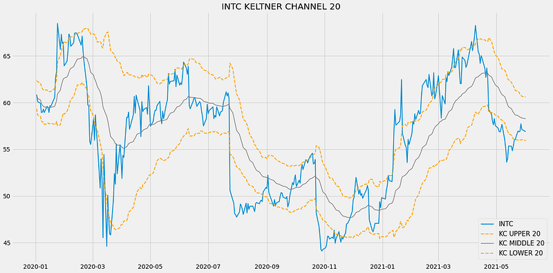
The above chart is a graphical representation of Intel’s 20-day Keltner Chanel. We could notice that two bands are plotted on either side of the closing price line and those are nothing but the upper and lower band and a grey-colored line running in-between the two bands is the middle line or the 20-day EMA. The Keltner Channel can be used in an extensive number of ways but the most popular usages are identifying the market volatility and direction.

The volatility of the market can be determined by the space that exists between the upper and lower band. If the space between the bands is wider, then the market is said to be volatile or showing greater price movements. On the other hand, the market is considered to be in a state of non-volatile or consolidating if the space between the bands is narrow. The other popular usage is identifying the market direction. The market direction can be determined by following the direction of the middle line as well as the upper and lower band.

While seeing the chart of the Keltner Channel, it might resemble the Bollinger Bands. The only difference between these two indicators is the way each of them is being calculated. The Bollinger Bands use standard deviation for its calculation, whereas, the Keltner Channel utilizes ATR to calculate its readings. Now, let’s talk about the trading strategy we are going to implement in this article.

About our trading strategy: We are going to implement the most popular Keltner Channel trading strategy which is the Breakout strategy. Since the Keltner Channel is prone to revealing false signals, we are going to tune the traditional breakout strategy. Our tuned strategy will reveal a buy signal whenever the closing price line crosses from above to below the lower band and the current closing price is lesser than the next closing price of the stock. Similarly, a sell signal is revealed whenever the closing price line crosses from below to above the upper band and the current closing price is greater than the next closing price of the stock. Our trading strategy can be represented as follows:

IF C.CLOSE < C.KCLOWER AND C.CLOSE < N.CLOSE ==> BUY SIGNAL
IF C.CLOSE > C.KCUPPER AND C.CLOSE > N.CLOSE ==> SELL SIGNAL

Many other strategies can also be implemented based on the Keltner Channel indicator but just to make things simple to understand, we are going with the breakout strategy. This concludes our theory part on the Keltner Channel indicator. Now, let’s move on to the programming part where we are first going to build the indicator from scratch, build the breakout strategy which we just discussed, then, compare our strategy’s performance with the SPY ETF’s returns in Python. Let’s do some coding! Before moving on, a note on disclaimer: This article’s sole purpose is to educate people and must be considered as an information piece but not as investment advice or so.

Implementation in Python

The coding part is classified into various steps as follows:

1. Importing Packages
2. Extracting Stock Data from EODHD
3. Keltner Channel Calculation
4. Creating the Breakout Trading Strategy
5. Plotting the Trading Lists
6. Creating our Position
7. Backtesting
8. SPY ETF Comparison

We will be following the order mentioned in the above list and buckle up your seat belts to follow every upcoming coding part.

Step-1: Importing Packages

Importing the required packages into the python environment is a non-skippable step. The primary packages are going to be Pandas to work with data, NumPy to work with arrays and for complex functions, Matplotlib for plotting purposes, and Requests to make API calls. The secondary packages are going to be Math for mathematical functions and Termcolor for font customization (optional).

Python Implementation:

# IMPORTING PACKAGES

import requests
import numpy as np
import matplotlib.pyplot as plt
import pandas as pd
from termcolor import colored as cl
from math import floor

plt.rcParams['figure.figsize'] = (20,10)
plt.style.use('fivethirtyeight')

With the required packages imported into Python, we can proceed to fetch historical data for Intel using EODHD’s OHLC split-adjusted data API endpoint.

Step-2: Extracting data from EODHD

In this phase, we’re set to retrieve the historical stock data for Intel using the OHLC split-adjusted API endpoint provided by EODHD. It’s important to note that EOD Historical Data (EODHD) is a reliable provider of financial APIs, encompassing an extensive array of market data, including historical data and economic news. Be sure to possess an EODHD account and access your secret API key, a crucial element for data extraction via the API.

Python Implementation:

# EXTRACTING STOCK DATA

def get_historical_data(symbol, start_date):
    api_key = 'YOUR API KEY'
    api_url = f'https://eodhistoricaldata.com/api/technical/{symbol}?order=a&fmt=json&from={start_date}&function=splitadjusted&api_token={api_key}'
    raw_df = requests.get(api_url).json()
    df = pd.DataFrame(raw_df)
    df.date = pd.to_datetime(df.date)
    df = df.set_index('date')
    return df

intc = get_historical_data('INTC', '2020-01-01')
intc.tail()

Output:

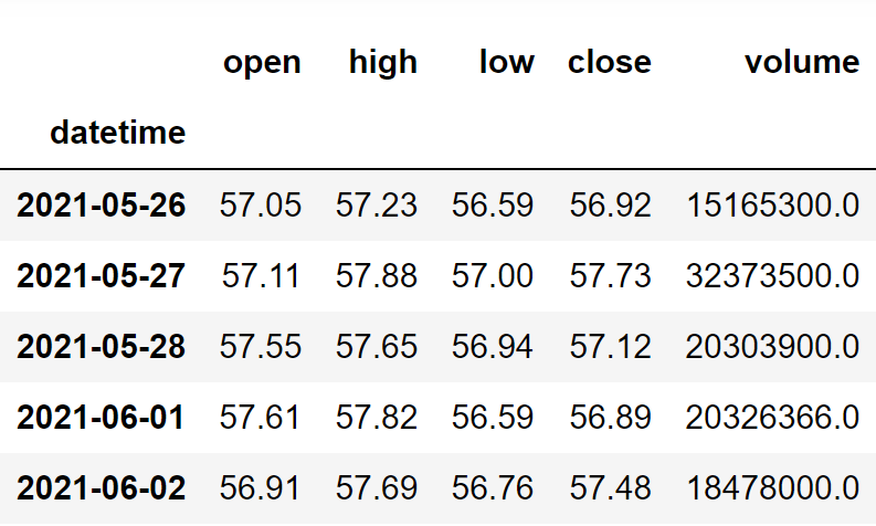
Code Explanation: We begin by defining a function named ‘get_historical_data,’ which takes the stock symbol (‘symbol’) and the start date for historical data (‘start_date’) as parameters. Inside the function, we define the API key and URL, then retrieve the historical data in JSON format using the ‘get’ function and store it in the ‘raw_df’ variable. After cleaning and formatting the raw JSON data, we return it as a Pandas dataframe. Finally, we call this function to fetch Intel’s historical data from the start of 2020 and store it in the ‘intc’ variable.

Step-3: Keltner Channel Calculation

In this step, we are going to calculate the components of the Keltner Channel indicator by following the methods we discussed before.

Python Implementation:

# KELTNER CHANNEL CALCULATION

def get_kc(high, low, close, kc_lookback, multiplier, atr_lookback):
    tr1 = pd.DataFrame(high - low)
    tr2 = pd.DataFrame(abs(high - close.shift()))
    tr3 = pd.DataFrame(abs(low - close.shift()))
    frames = [tr1, tr2, tr3]
    tr = pd.concat(frames, axis = 1, join = 'inner').max(axis = 1)
    atr = tr.ewm(alpha = 1/atr_lookback).mean()
    
    kc_middle = close.ewm(kc_lookback).mean()
    kc_upper = close.ewm(kc_lookback).mean() + multiplier * atr
    kc_lower = close.ewm(kc_lookback).mean() - multiplier * atr
    
    return kc_middle, kc_upper, kc_lower
    
intc = intc.iloc[:,:4]
intc['kc_middle'], intc['kc_upper'], intc['kc_lower'] = get_kc(intc['high'], intc['low'], intc['close'], 20, 2, 10)
intc.tail()

Output:

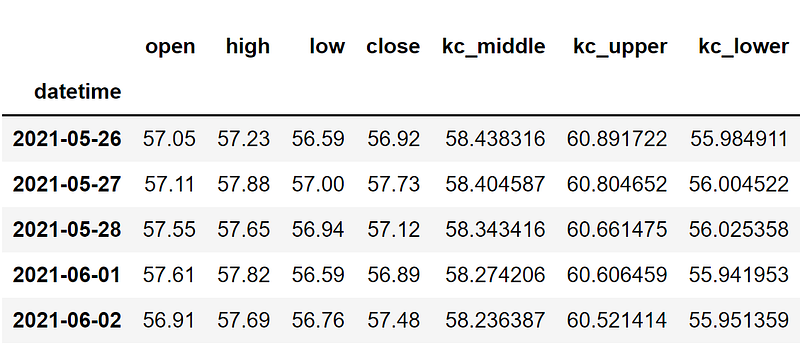
Code Explanation: We are first defining a function named ‘get_kc’ that takes a stock’s high (‘high’), low (‘low’), and closing price data (‘close’), the lookback period for the Keltner Channel (‘kc_lookback’), the multiplier value (‘multiplier), and the lookback period for the ATR (‘atr_lookback’) as parameters. The code inside the function can be separated into two parts: ATR calculation, and the Keltner Channel calculation.

ATR calculation: To determine the readings of the Average True Range, we are first calculating the three differences and stored them into their respective variables. Then we are combining all three differences into one dataframe using the ‘concat’ function and took the maximum values out of the three collective differences to determine the True Range. Then, using the ‘ewm’ and ‘mean’ functions, we are taking the customized Moving Average of True Range for a specified number of periods to get the ATR values.

Keltner Channel calculation: Utilizing the previously calculated ATR values, we are first calculating the middle line of the Keltner Channel by taking the EMA of ATR for a specified number of periods. Then comes the calculation of both the upper and lower bands. We are substituting the ATR values into the upper and lower bands formula we discussed before to get the readings of each of them. Finally, we are returning and calling the created function to get the Keltner Channel values of Intel.

Step-4: Creating the trading strategy

In this step, we are going to implement the discussed Keltner Channel indicator breakout trading strategy in python.

Python Implementation:

# KELTNER CHANNEL STRATEGY

def implement_kc_strategy(prices, kc_upper, kc_lower):
    buy_price = []
    sell_price = []
    kc_signal = []
    signal = 0
    
    for i in range(len(prices)):
        if prices[i] < kc_lower[i] and prices[i+1] > prices[i]:
            if signal != 1:
                buy_price.append(prices[i])
                sell_price.append(np.nan)
                signal = 1
                kc_signal.append(signal)
            else:
                buy_price.append(np.nan)
                sell_price.append(np.nan)
                kc_signal.append(0)
        elif prices[i] > kc_upper[i] and prices[i+1] < prices[i]:
            if signal != -1:
                buy_price.append(np.nan)
                sell_price.append(prices[i])
                signal = -1
                kc_signal.append(signal)
            else:
                buy_price.append(np.nan)
                sell_price.append(np.nan)
                kc_signal.append(0)
        else:
            buy_price.append(np.nan)
            sell_price.append(np.nan)
            kc_signal.append(0)
            
    return buy_price, sell_price, kc_signal

buy_price, sell_price, kc_signal = implement_kc_strategy(intc['close'], intc['kc_upper'], intc['kc_lower'])

Code Explanation: First, we are defining a function named ‘implement_kc_strategy’ which takes the stock prices (‘prices’), and the components of the Keltner Channel indicator (‘kc_upper’, and ‘kc_lower’) as parameters.

Inside the function, we are creating three empty lists (buy_price, sell_price, and kc_signal) in which the values will be appended while creating the trading strategy.

After that, we are implementing the trading strategy through a for-loop. Inside the for-loop, we are passing certain conditions, and if the conditions are satisfied, the respective values will be appended to the empty lists. If the condition to buy the stock gets satisfied, the buying price will be appended to the ‘buy_price’ list, and the signal value will be appended as 1 representing to buy the stock. Similarly, if the condition to sell the stock gets satisfied, the selling price will be appended to the ‘sell_price’ list, and the signal value will be appended as -1 representing to sell the stock.

Finally, we are returning the lists appended with values. Then, we are calling the created function and stored the values into their respective variables. The list doesn’t make any sense unless we plot the values. So, let’s plot the values of the created trading lists.

Step-5: Plotting the trading signals

In this step, we are going to plot the created trading lists to make sense out of them.

Python Implementation:

# TRADING SIGNALS PLOT

plt.plot(intc['close'], linewidth = 2, label = 'INTC')
plt.plot(intc['kc_upper'], linewidth = 2, color = 'orange', linestyle = '--', label = 'KC UPPER 20')
plt.plot(intc['kc_middle'], linewidth = 1.5, color = 'grey', label = 'KC MIDDLE 20')
plt.plot(intc['kc_lower'], linewidth = 2, color = 'orange', linestyle = '--', label = 'KC LOWER 20')
plt.plot(intc.index, buy_price, marker = '^', color = 'green', markersize = 15, linewidth = 0, label = 'BUY SIGNAL')
plt.plot(intc.index, sell_price, marker = 'v', color= 'r', markersize = 15, linewidth = 0, label = 'SELL SIGNAL')
plt.legend(loc = 'lower right')
plt.title('INTC KELTNER CHANNEL 20 TRADING SIGNALS')
plt.show()

Output:

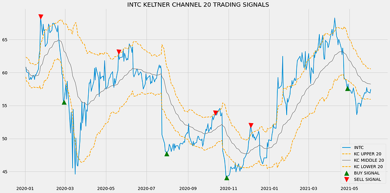
Code Explanation: We are plotting the readings of the components of the Keltner Channel indicator along with the buy and sell signals generated by the breakout trading strategy. We can observe that whenever the closing price line from above to below the lower band line and the current closing price is lower than the next closing price, a green-colored buy signal is plotted in the chart. Similarly, whenever the closing price line crosses from below to above the upper band and the current closing price is greater than the next closing price, a red-colored sell signal is plotted in the chart.

Step-6: Creating our Position

In this step, we are going to create a list that indicates 1 if we hold the stock or 0 if we don’t own or hold the stock.

Python Implementation:

# STOCK POSITION

position = []
for i in range(len(kc_signal)):
    if kc_signal[i] > 1:
        position.append(0)
    else:
        position.append(1)
        
for i in range(len(intc['close'])):
    if kc_signal[i] == 1:
        position[i] = 1
    elif kc_signal[i] == -1:
        position[i] = 0
    else:
        position[i] = position[i-1]
        
close_price = intc['close']
kc_upper = intc['kc_upper']
kc_lower = intc['kc_lower']
kc_signal = pd.DataFrame(kc_signal).rename(columns = {0:'kc_signal'}).set_index(intc.index)
position = pd.DataFrame(position).rename(columns = {0:'kc_position'}).set_index(intc.index)

frames = [close_price, kc_upper, kc_lower, kc_signal, position]
strategy = pd.concat(frames, join = 'inner', axis = 1)

strategy

Output:

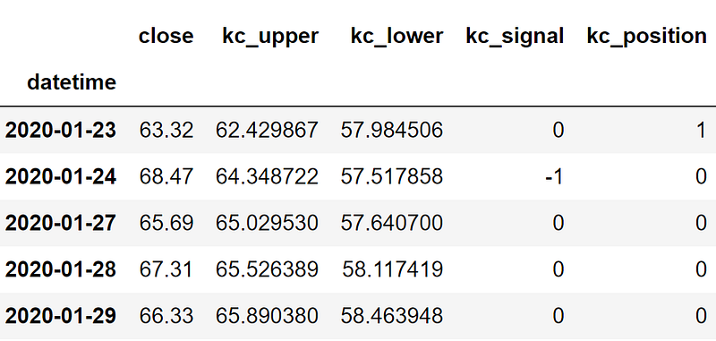
Code Explanation: First, we are creating an empty list named ‘position’. We are passing two for-loops, one is to generate values for the ‘position’ list to just match the length of the ‘signal’ list. The other for-loop is the one we are using to generate actual position values. Inside the second for-loop, we are iterating over the values of the ‘signal’ list, and the values of the ‘position’ list get appended concerning which condition gets satisfied. The value of the position remains 1 if we hold the stock or remains 0 if we sold or don’t own the stock. Finally, we are doing some data manipulations to combine all the created lists into one dataframe.

From the output being shown, we can see that in the first row our position in the stock has remained 1 (since there isn’t any change in the Keltner Channel indicator signal) but our position suddenly turned to -1 as we sold the stock when the Keltner Channel indicator trading signal represents a sell signal (-1). Our position will remain 0 until some changes in the trading signal occur. Now it’s time to do implement some backtesting process!

Step-7: Backtesting

Before moving on, it is essential to know what backtesting is. Backtesting is the process of seeing how well our trading strategy has performed on the given stock data. In our case, we are going to implement a backtesting process for our Keltner Channel indicator trading strategy over the Intel stock data.

Python Implementation:

# BACKTESTING

intc_ret = pd.DataFrame(np.diff(intc['close'])).rename(columns = {0:'returns'})
kc_strategy_ret = []

for i in range(len(intc_ret)):
    returns = intc_ret['returns'][i]*strategy['kc_position'][i]
    kc_strategy_ret.append(returns)
    
kc_strategy_ret_df = pd.DataFrame(kc_strategy_ret).rename(columns = {0:'kc_returns'})
investment_value = 100000
number_of_stocks = floor(investment_value/intc['close'][0])
kc_investment_ret = []

for i in range(len(kc_strategy_ret_df['kc_returns'])):
    returns = number_of_stocks*kc_strategy_ret_df['kc_returns'][i]
    kc_investment_ret.append(returns)

kc_investment_ret_df = pd.DataFrame(kc_investment_ret).rename(columns = {0:'investment_returns'})
total_investment_ret = round(sum(kc_investment_ret_df['investment_returns']), 2)
profit_percentage = floor((total_investment_ret/investment_value)*100)
print(cl('Profit gained from the KC strategy by investing $100k in INTC : {}'.format(total_investment_ret), attrs = ['bold']))
print(cl('Profit percentage of the KC strategy : {}%'.format(profit_percentage), attrs = ['bold']))

Output:

Profit gained from the KC strategy by investing $100k in INTC : 47786.65
Profit percentage of the KC strategy : 47%

Code Explanation: First, we are calculating the returns of the Intel stock using the ‘diff’ function provided by the NumPy package and we have stored it as a dataframe into the ‘intc_ret’ variable. Next, we are passing a for-loop to iterate over the values of the ‘intc_ret’ variable to calculate the returns we gained from our Keltner Channel indicator trading strategy, and these returns values are appended to the ‘kc_strategy_ret’ list. Next, we are converting the ‘kc_strategy_ret’ list into a dataframe and stored it into the ‘kc_strategy_ret_df’ variable.

Next comes the backtesting process. We are going to backtest our strategy by investing a hundred thousand USD into our trading strategy. So first, we are storing the amount of investment into the ‘investment_value’ variable. After that, we are calculating the number of Intel stocks we can buy using the investment amount. You can notice that I’ve used the ‘floor’ function provided by the Math package because, while dividing the investment amount by the closing price of Intel stock, it spits out an output with decimal numbers. The number of stocks should be an integer but not a decimal number. Using the ‘floor’ function, we can cut out the decimals. Remember that the ‘floor’ function is way more complex than the ‘round’ function. Then, we are passing a for-loop to find the investment returns followed by some data manipulation tasks.

Finally, we are printing the total return we got by investing a hundred thousand into our trading strategy and it is revealed that we have made an approximate profit of forty-seven thousand USD in one year. That’s not bad! Now, let’s compare our returns with SPY ETF (an ETF designed to track the S&P 500 stock market index) returns.

Step-8: SPY ETF Comparison

This step is optional but it is highly recommended as we can get an idea of how well our trading strategy performs against a benchmark (SPY ETF). In this step, we are going to extract the data of the SPY ETF using the ‘get_historical_data’ function we created and compare the returns we get from the SPY ETF with our Keltner Channel breakout trading strategy returns on Intel.

You might have observed that in all of my algorithmic trading articles, I’ve compared the strategy results not with the S&P 500 market index itself but with the SPY ETF and this is because most of the stock data providers (like Twelve Data) don’t provide the S&P 500 index data. So, I have no other choice than to go with the SPY ETF. If you’re fortunate to get the S&P 500 market index data, it is recommended to use it for comparison rather than any ETF.

Python Implementation:

# SPY ETF COMPARISON

def get_benchmark(start_date, investment_value):
    spy = get_historical_data('SPY', start_date)['close']
    benchmark = pd.DataFrame(np.diff(spy)).rename(columns = {0:'benchmark_returns'})
    
    investment_value = investment_value
    number_of_stocks = floor(investment_value/spy[-1])
    benchmark_investment_ret = []
    
    for i in range(len(benchmark['benchmark_returns'])):
        returns = number_of_stocks*benchmark['benchmark_returns'][i]
        benchmark_investment_ret.append(returns)

    benchmark_investment_ret_df = pd.DataFrame(benchmark_investment_ret).rename(columns = {0:'investment_returns'})
    return benchmark_investment_ret_df

benchmark = get_benchmark('2020-01-01', 100000)
investment_value = 100000
total_benchmark_investment_ret = round(sum(benchmark['investment_returns']), 2)
benchmark_profit_percentage = floor((total_benchmark_investment_ret/investment_value)*100)
print(cl('Benchmark profit by investing $100k : {}'.format(total_benchmark_investment_ret), attrs = ['bold']))
print(cl('Benchmark Profit percentage : {}%'.format(benchmark_profit_percentage), attrs = ['bold']))
print(cl('KC Strategy profit is {}% higher than the Benchmark Profit'.format(profit_percentage - benchmark_profit_percentage), attrs = ['bold']))

Output:

Benchmark profit by investing $100k : 22631.16
Benchmark Profit percentage : 22%
KC Strategy profit is 25% higher than the Benchmark Profit

Code Explanation: The code used in this step is almost similar to the one used in the previous backtesting step but, instead of investing in Intel, we are investing in SPY ETF by not implementing any trading strategies. From the output, we can see that our Keltner Channel breakout trading strategy has outperformed the SPY ETF by 25%. That’s great!

Final Thoughts!

After a long process of crushing both theory and coding parts, we have successfully learned what the Keltner Channel indicator is all about, the math behind the indicator, and finally, how to build the indicator from scratch and construct the breakout trading strategy in Python. We also did manage to get some nice results and in fact, apart from surpassing the returns of the SPY ETF, we exceeded the actual Intel stock returns itself with our breakout strategy.

I often talk about strategy tuning or optimization in my articles and today, we really did implemented it by tuning and making some changes to the traditional breakout strategy. As a result, we were able to outdo the returns of the actual market itself. This is just one small example of how to tune a strategy and how the results will be impacted accordingly but, there is a lot more to be explored. Strategy optimization is not only about tuning or making some changes to the traditional strategies that exist for a long time but about creating an optimal trading environment and this includes the broker you are using for trading purposes, the risk management system, and so on. So it’s highly recommended to have a look at these spaces to take your strategies to a whole new level.

With that being said, you have reached the end of the article. If you forgot to follow any of the coding parts, don’t worry. I’ve provided the full source code at the end. Hope you learned something new and useful from this article.

Full code:

# IMPORTING PACKAGES

import requests
import numpy as np
import matplotlib.pyplot as plt
import pandas as pd
from termcolor import colored as cl
from math import floor

plt.rcParams['figure.figsize'] = (20,10)
plt.style.use('fivethirtyeight')


# EXTRACTING STOCK DATA

def get_historical_data(symbol, start_date):
    api_key = 'YOUR API KEY'
    api_url = f'https://api.twelvedata.com/time_series?symbol={symbol}&interval=1day&outputsize=5000&apikey={api_key}'
    raw_df = requests.get(api_url).json()
    df = pd.DataFrame(raw_df['values']).iloc[::-1].set_index('datetime').astype(float)
    df = df[df.index >= start_date]
    df.index = pd.to_datetime(df.index)
    return df

intc = get_historical_data('INTC', '2020-01-01')
print(intc.tail())


# KELTNER CHANNEL CALCULATION

def get_kc(high, low, close, kc_lookback, multiplier, atr_lookback):
    tr1 = pd.DataFrame(high - low)
    tr2 = pd.DataFrame(abs(high - close.shift()))
    tr3 = pd.DataFrame(abs(low - close.shift()))
    frames = [tr1, tr2, tr3]
    tr = pd.concat(frames, axis = 1, join = 'inner').max(axis = 1)
    atr = tr.ewm(alpha = 1/atr_lookback).mean()
    
    kc_middle = close.ewm(kc_lookback).mean()
    kc_upper = close.ewm(kc_lookback).mean() + multiplier * atr
    kc_lower = close.ewm(kc_lookback).mean() - multiplier * atr
    
    return kc_middle, kc_upper, kc_lower
    
intc = intc.iloc[:,:4]
intc['kc_middle'], intc['kc_upper'], intc['kc_lower'] = get_kc(intc['high'], intc['low'], intc['close'], 20, 2, 10)
print(intc.tail())


# KELTNER CHANNEL PLOT

plt.plot(intc['close'], linewidth = 2, label = 'INTC')
plt.plot(intc['kc_upper'], linewidth = 2, color = 'orange', linestyle = '--', label = 'KC UPPER 20')
plt.plot(intc['kc_middle'], linewidth = 1.5, color = 'grey', label = 'KC MIDDLE 20')
plt.plot(intc['kc_lower'], linewidth = 2, color = 'orange', linestyle = '--', label = 'KC LOWER 20')
plt.legend(loc = 'lower right', fontsize = 15)
plt.title('INTC KELTNER CHANNEL 20')
plt.show()


# KELTNER CHANNEL STRATEGY

def implement_kc_strategy(prices, kc_upper, kc_lower):
    buy_price = []
    sell_price = []
    kc_signal = []
    signal = 0
    
    for i in range(len(prices)):
        if prices[i] < kc_lower[i] and prices[i+1] > prices[i]:
            if signal != 1:
                buy_price.append(prices[i])
                sell_price.append(np.nan)
                signal = 1
                kc_signal.append(signal)
            else:
                buy_price.append(np.nan)
                sell_price.append(np.nan)
                kc_signal.append(0)
        elif prices[i] > kc_upper[i] and prices[i+1] < prices[i]:
            if signal != -1:
                buy_price.append(np.nan)
                sell_price.append(prices[i])
                signal = -1
                kc_signal.append(signal)
            else:
                buy_price.append(np.nan)
                sell_price.append(np.nan)
                kc_signal.append(0)
        else:
            buy_price.append(np.nan)
            sell_price.append(np.nan)
            kc_signal.append(0)
            
    return buy_price, sell_price, kc_signal

buy_price, sell_price, kc_signal = implement_kc_strategy(intc['close'], intc['kc_upper'], intc['kc_lower'])


# TRADING SIGNALS PLOT

plt.plot(intc['close'], linewidth = 2, label = 'INTC')
plt.plot(intc['kc_upper'], linewidth = 2, color = 'orange', linestyle = '--', label = 'KC UPPER 20')
plt.plot(intc['kc_middle'], linewidth = 1.5, color = 'grey', label = 'KC MIDDLE 20')
plt.plot(intc['kc_lower'], linewidth = 2, color = 'orange', linestyle = '--', label = 'KC LOWER 20')
plt.plot(intc.index, buy_price, marker = '^', color = 'green', markersize = 15, linewidth = 0, label = 'BUY SIGNAL')
plt.plot(intc.index, sell_price, marker = 'v', color= 'r', markersize = 15, linewidth = 0, label = 'SELL SIGNAL')
plt.legend(loc = 'lower right')
plt.title('INTC KELTNER CHANNEL 20 TRADING SIGNALS')
plt.show()


# STOCK POSITION

position = []
for i in range(len(kc_signal)):
    if kc_signal[i] > 1:
        position.append(0)
    else:
        position.append(1)
        
for i in range(len(intc['close'])):
    if kc_signal[i] == 1:
        position[i] = 1
    elif kc_signal[i] == -1:
        position[i] = 0
    else:
        position[i] = position[i-1]
        
close_price = intc['close']
kc_upper = intc['kc_upper']
kc_lower = intc['kc_lower']
kc_signal = pd.DataFrame(kc_signal).rename(columns = {0:'kc_signal'}).set_index(intc.index)
position = pd.DataFrame(position).rename(columns = {0:'kc_position'}).set_index(intc.index)

frames = [close_price, kc_upper, kc_lower, kc_signal, position]
strategy = pd.concat(frames, join = 'inner', axis = 1)

print(strategy)
print(strategy[14:19])


# BACKTESTING

intc_ret = pd.DataFrame(np.diff(intc['close'])).rename(columns = {0:'returns'})
kc_strategy_ret = []

for i in range(len(intc_ret)):
    returns = intc_ret['returns'][i]*strategy['kc_position'][i]
    kc_strategy_ret.append(returns)
    
kc_strategy_ret_df = pd.DataFrame(kc_strategy_ret).rename(columns = {0:'kc_returns'})
investment_value = 100000
number_of_stocks = floor(investment_value/intc['close'][0])
kc_investment_ret = []

for i in range(len(kc_strategy_ret_df['kc_returns'])):
    returns = number_of_stocks*kc_strategy_ret_df['kc_returns'][i]
    kc_investment_ret.append(returns)

kc_investment_ret_df = pd.DataFrame(kc_investment_ret).rename(columns = {0:'investment_returns'})
total_investment_ret = round(sum(kc_investment_ret_df['investment_returns']), 2)
profit_percentage = floor((total_investment_ret/investment_value)*100)
print(cl('Profit gained from the KC strategy by investing $100k in INTC : {}'.format(total_investment_ret), attrs = ['bold']))
print(cl('Profit percentage of the KC strategy : {}%'.format(profit_percentage), attrs = ['bold']))


# SPY ETF COMPARISON

def get_benchmark(start_date, investment_value):
    spy = get_historical_data('SPY', start_date)['close']
    benchmark = pd.DataFrame(np.diff(spy)).rename(columns = {0:'benchmark_returns'})
    
    investment_value = investment_value
    number_of_stocks = floor(investment_value/spy[-1])
    benchmark_investment_ret = []
    
    for i in range(len(benchmark['benchmark_returns'])):
        returns = number_of_stocks*benchmark['benchmark_returns'][i]
        benchmark_investment_ret.append(returns)

    benchmark_investment_ret_df = pd.DataFrame(benchmark_investment_ret).rename(columns = {0:'investment_returns'})
    return benchmark_investment_ret_df

benchmark = get_benchmark('2020-01-01', 100000)
investment_value = 100000
total_benchmark_investment_ret = round(sum(benchmark['investment_returns']), 2)
benchmark_profit_percentage = floor((total_benchmark_investment_ret/investment_value)*100)
print(cl('Benchmark profit by investing $100k : {}'.format(total_benchmark_investment_ret), attrs = ['bold']))
print(cl('Benchmark Profit percentage : {}%'.format(benchmark_profit_percentage), attrs = ['bold']))
print(cl('KC Strategy profit is {}% higher than the Benchmark Profit'.format(profit_percentage - benchmark_profit_percentage), attrs = ['bold']))