This content discusses a strategy for predicting JPM stock prices using a combination of autoregressive, Fourier, and deep learning models, along with technical indicators, for robust stock price prediction and backtesting.
Abstract
The content focuses on a holistic strategy for predicting JPM stock prices using a combination of autoregressive, Fourier, and deep learning models, along with technical indicators. The approach aims to integrate predictive analytics and technical indicators into a single decision-making framework for detecting and predicting financial asset price breakouts and trends. The ultimate goal is to apply financial risk management to stock trading and investments, maximizing ROI while minimizing the likelihood of losing money on investment decisions. The content also discusses the use of SaaS products to automate trading and generate profits at a speed and frequency unattainable for human traders.
Opinions
The content emphasizes the importance of integrating predictive analytics and technical indicators into a single decision-making framework for stock price prediction and backtesting.
The authors believe that a combination of autoregressive, Fourier, and deep learning models, along with technical indicators, can provide a more robust and accurate prediction of stock prices.
The authors argue that the use of SaaS products to automate trading can generate profits at a speed and frequency unattainable for human traders.
The authors suggest that the ultimate goal of algorithmic trading is to apply financial risk management to stock trading and investments, maximizing ROI while minimizing the likelihood of losing money on investment decisions.
The authors highlight the importance of calculating and comparing risk-adjusted returns, beta, annual volatility, and standard deviation against the S&P 500 benchmark to maximize the (ROI/Risk) ratio.
The authors predict that the key trends, case examples, and best industry practices will accelerate the algorithmic trading market growth in the near future.
The authors suggest that factors such as the increasing adoption of ML/AI, real-time data analytics, interactive visualizations, and the rising demand for automated trading systems substantiate the current rapid algorithmic trading industry growth in North America, Europe, and Asia.
Combining ARIMA, LSTM and Fourier Models with Technical Indicators for JPM Price Prediction and Backtesting
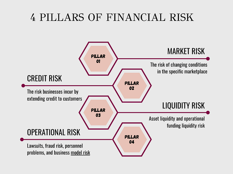
Four Pillars of Financial Risk: Market Risk, Credit Risk, Liquidity Risk, and Operational Risk
Business Motivation: Banks have always been vulnerable to quickly shifting sentiment among investors, depositors, and regulators. In the year since authorities in the U.S. and Switzerland stepped in to quell contagion risk after the collapse of SVB, Signature, and Credit Suisse, regulators remain acutely aware of the sector’s sensitivities.
Unlike other papers that concentrate on a one-size-fits-all technique, in this paper we follow a more holistic strategy that integrates predictive analytics and TI into a single decision-making framework aimed at detecting and predicting financial asset price breakouts and trends to make informed decisions.
The ultimate business goal of AT is the systematic application of Financial Risk Management to stock (algorithmic) trading and investments. In fact, traders always strive to maximize ROI while minimizing the likelihood of losing money on investment decisions. This is where AT comes into play.
Simply put, AT is when you use SaaS products to open and close trades according to set rules such as points of price movement in an underlying market. Once the current market conditions match any predetermined criteria, trading algorithms (algos) can execute a buy or sell order on your behalf.
In principle, AT can generate profits at a speed and frequency that is impossible for a human trader. To earn profits at an unattainable frequency for a human trader, algorithms are used to automate trading.
While TI-powered technical analysis is just one approach to risk-aware time-series analysis, it can complement other quantitative methods such as statistical/ML price forecasting and provide credible fintech BI insights into securities.
Let’s dive into further details of this integrated model-based TI methodology.
Setting the working directory YOURPATH and importing/installing Python libraries
import os
os.chdir('YOURPATH') # Set working directory
os. getcwd()
!pip install pmdarima, yfinance, statsmodels, matplotlib, sklearn, keras,quantstats
import yfinance as yf
import pandas as pd
import numpy as np
from pmdarima.arima import auto_arima
from statsmodels.tsa.arima.model import ARIMA
import matplotlib.pyplot as plt
from pandas_datareader.data import DataReader
from pandas_datareader import data as pdr
from keras.models import Sequential
from keras.layers import Dense, LSTM
# For time stampsfrom datetime import datetime
from datetime import datetime as dt, timedelta as td
import quantstats as qs
from sklearn.preprocessing import MinMaxScaler
from sklearn.metrics import mean_squared_error,mean_absolute_error,explained_variance_score,r2_score
Reading Input Stock Data
Option 1: Use yf.download
# Download data
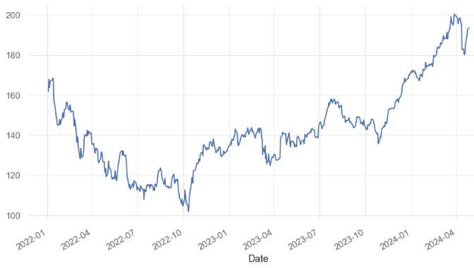
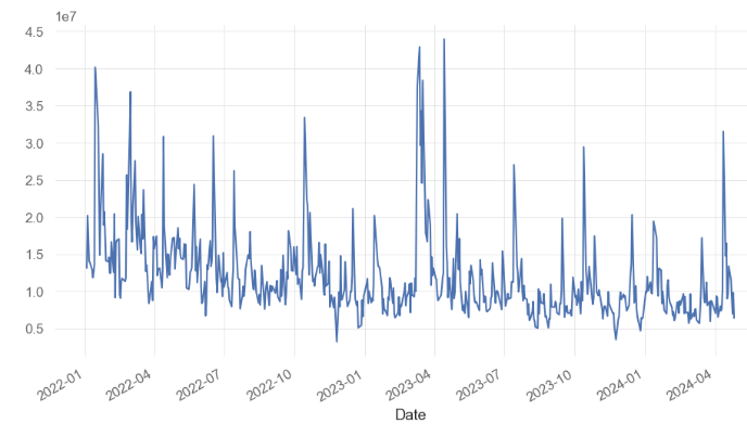
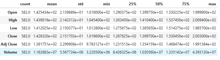
gs = yf.download("JPM", start="2022-01-03", end="2024-04-26")
gs
Open High Low Close Adj Close Volume
Date
2022-01-03 159.860001162.639999159.509995161.699997150.404938131209002022-01-04 164.309998168.580002164.229996167.830002156.106750201958002022-01-05 167.820007168.360001163.729996163.779999153.252762175394002022-01-06 166.910004167.369995163.869995165.520004154.880951140475002022-01-07 165.669998167.529999165.059998167.160004156.41554313913300... ... ... ... ... ... ...
2024-04-22185.990005190.130005185.979996189.410004189.410004115297002024-04-23191.130005192.229996190.520004192.139999192.13999991444002024-04-24190.529999193.229996190.169998193.080002193.08000269649002024-04-25192.250000193.940002191.179993193.369995193.36999598023002024-04-26193.570007194.869995193.059998193.490005193.4900056408600582 rows × 6 columns
defget_sharpe(stock):
start=dt.today()-td(365*2)
df = yf.download(stock,start=start)['Adj Close']
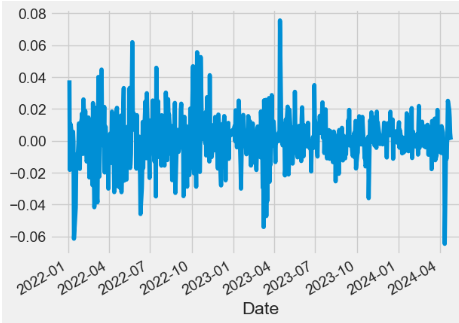
ret = df.pct_change()
ri = ret.mean()
rf = (.0467 / 365) # 10 Year Treasury Rate of 4.67% for Apr 26 2024
sigma = ret.std()
sr = (ri - rf) * 250 ** .5 / sigma # annualize the sharpe ratioprint(f'Sharpe Ratio of {stock.upper()} is : {sr}')
return sr
get_sharpe('JPM')
Sharpe Ratio of JPM is : 1.13994216822035
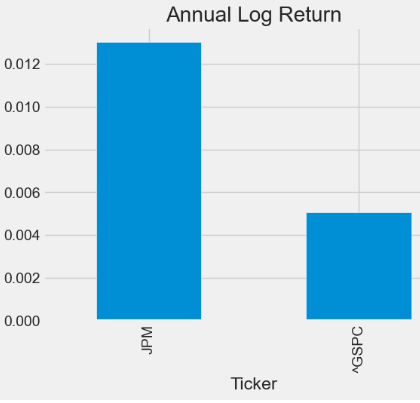
Comparing 2Y kurtosis, skewness and std: JPM vs ^GSPC benchmark
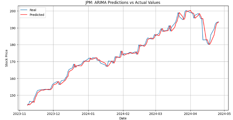
Running ARIMA model forecasting with 80:20 % train/test split
# Define the ARIMA modeldefarima_forecast(history):
# Fit the model
model = ARIMA(history, order=(0,1,0))
model_fit = model.fit()
# Make the prediction
output = model_fit.forecast()
yhat = output[0]
return yhat
# Split data into train and test sets
X = dataset_ex_df.values
size = int(len(X) * 0.8)
train, test = X[0:size], X[size:len(X)]
# Walk-forward validation
history = [x for x in train]
predictions = list()
for t inrange(len(test)):
# Generate a prediction
yhat = arima_forecast(history)
predictions.append(yhat)
# Add the predicted value to the training set
obs = test[t]
history.append(obs)
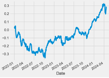
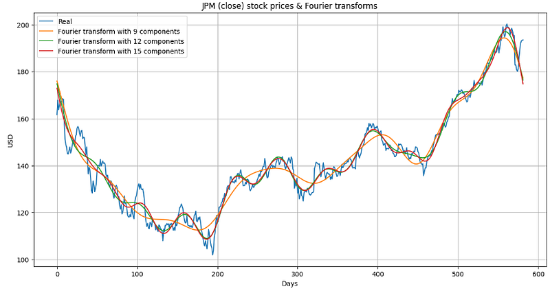
By applying FFT to stock market data, we can decompose the data into its harmonic components and examine trends, cycles, and other patterns in the data that may not be apparent by simply looking at the time-domain stock prices.
# Create a new dataframe with only the 'Close column
data = df.filter(['Close'])
# Convert the dataframe to a numpy array
dataset = data.values
# Get the number of rows to train the model on
training_data_len = int(np.ceil( len(dataset) * .95 ))
training_data_len
553# Scale the data
scaler = MinMaxScaler(feature_range=(0,1))
scaled_data = scaler.fit_transform(dataset)
# Create the scaled training data set
train_data = scaled_data[0:int(training_data_len), :]
# Split the data into x_train and y_train data sets
x_train = []
y_train = []
for i inrange(60, len(train_data)):
x_train.append(train_data[i-60:i, 0])
y_train.append(train_data[i, 0])
if i<= 61:
print(x_train)
print(y_train)
print()
# Convert the x_train and y_train to numpy arrays
x_train, y_train = np.array(x_train), np.array(y_train)
# Reshape the data
x_train = np.reshape(x_train, (x_train.shape[0], x_train.shape[1], 1))
Building, compiling and running the LSTM model
from keras.models import Sequential
from keras.layers import Dense, LSTM
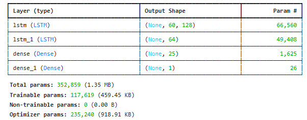
# Build the LSTM model
model = Sequential()
model.add(LSTM(128, return_sequences=True, input_shape= (x_train.shape[1], 1)))
model.add(LSTM(64, return_sequences=False))
model.add(Dense(25))
model.add(Dense(1))
# Compile the model
model.compile(optimizer='adam', loss='mean_squared_error')
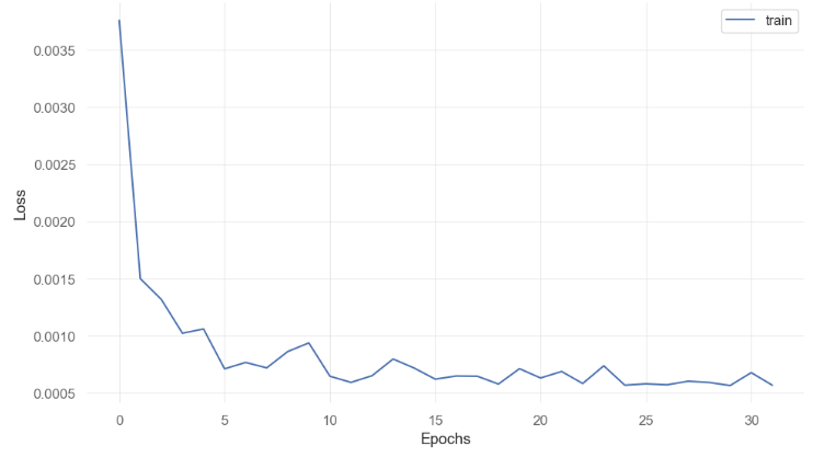
# Train the model
history=model.fit(x_train, y_train, batch_size=1, epochs=32)
493/493 ━━━━━━━━━━━━━━━━━━━━ 8s 12ms/step - loss: 0.0067
Epoch 2/32
..................
Epoch 30/32493/493 ━━━━━━━━━━━━━━━━━━━━ 7s 15ms/step - loss: 5.1676e-04
# Create a new array containing scaled values from index 1543 to 2002
test_data = scaled_data[training_data_len - 60: , :]
# Create the data sets x_test and y_test
x_test = []
y_test = dataset[training_data_len:, :]
for i inrange(60, len(test_data)):
x_test.append(test_data[i-60:i, 0])
# Convert the data to a numpy array
x_test = np.array(x_test)
# Reshape the data
x_test = np.reshape(x_test, (x_test.shape[0], x_test.shape[1], 1 ))
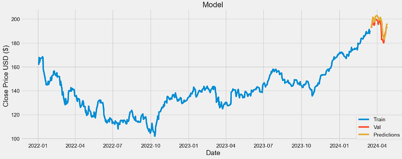
# Get the models predicted price values
predictions = model.predict(x_test)
predictions = scaler.inverse_transform(predictions)
# Get the root mean squared error (RMSE)
rmse = np.sqrt(np.mean(((predictions - y_test) ** 2)))
rmse
4.21706997838837
We have addressed a very challenging task of predicting trends in JPM prices and calculating future value of this asset.
We believe that the well known challenges of highly volatile and dynamic financial markets can be reduced by incorporating model-based time-series forecasting methods, fintech data analytics and TI-powered stock screening into a single Python-based algo-trading (AT) platform.
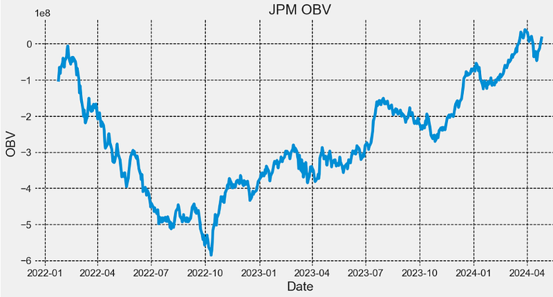
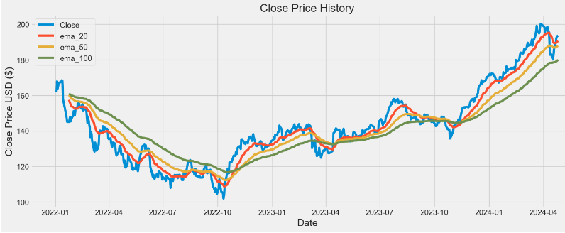
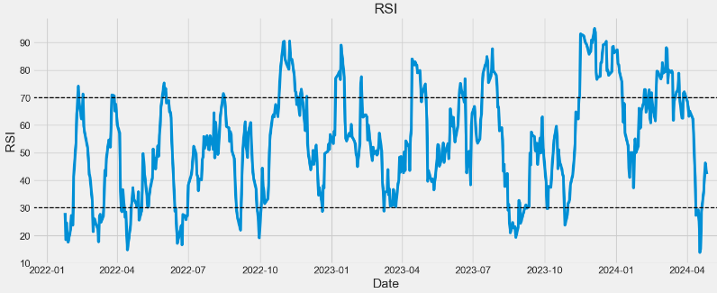
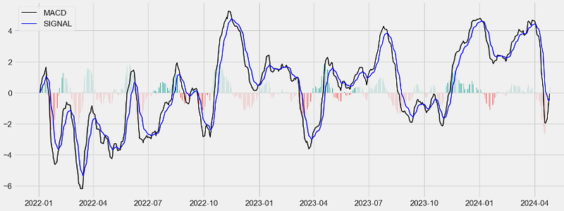
This paper proposes trading strategies based on quantitative analysis of time series data using ARIMA, FFT, LSTM, and popular TI such as EMA, RSI, MACD, and OBV.
We have also calculated and compared against the S&P 500 benchmark the JPM risk-adjusted returns, beta, annual volatility and std aimed at maximizing the (ROI/Risk) ratio.
The Road Ahead: we will continue looking at the key trends, case examples and best industry practices that set to accelerate the AT market growth in the near future. Factors such as the increasing adoption of ML/AI, real-time data analytics, interactive visualizations, and the rising demand for automated trading systems do substantiate the current rapid AT industry growth in 3 key regions such as North America, Europe, and Asia.