Free AI web copilot to create summaries, insights and extended knowledge, download it at here
7808
Abstract
ation & Plot</li></ul><div id="2ad3"><pre><span class="hljs-comment"># ADX CALCULATION</span>
<span class="hljs-keyword">def</span> <span class="hljs-title function_">get_adx</span>(<span class="hljs-params">high, low, close, lookback</span>):
plus_dm = high.diff()
minus_dm = low.diff()
plus_dm[plus_dm < <span class="hljs-number">0</span>] = <span class="hljs-number">0</span>
minus_dm[minus_dm > <span class="hljs-number">0</span>] = <span class="hljs-number">0</span>
tr1 = pd.DataFrame(high - low)
tr2 = pd.DataFrame(<span class="hljs-built_in">abs</span>(high - close.shift(<span class="hljs-number">1</span>)))
tr3 = pd.DataFrame(<span class="hljs-built_in">abs</span>(low - close.shift(<span class="hljs-number">1</span>)))
frames = [tr1, tr2, tr3]
tr = pd.concat(frames, axis = <span class="hljs-number">1</span>, join = <span class="hljs-string">'inner'</span>).<span class="hljs-built_in">max</span>(axis = <span class="hljs-number">1</span>)
atr = tr.rolling(lookback).mean()

plus_di = <span class="hljs-number">100</span> * (plus_dm.ewm(alpha = <span class="hljs-number">1</span>/lookback).mean() / atr)
minus_di = <span class="hljs-built_in">abs</span>(<span class="hljs-number">100</span> * (minus_dm.ewm(alpha = <span class="hljs-number">1</span>/lookback).mean() / atr))
dx = (<span class="hljs-built_in">abs</span>(plus_di - minus_di) / <span class="hljs-built_in">abs</span>(plus_di + minus_di)) * <span class="hljs-number">100</span>
adx = ((dx.shift(<span class="hljs-number">1</span>) * (lookback - <span class="hljs-number">1</span>)) + dx) / lookback
adx_smooth = adx.ewm(alpha = <span class="hljs-number">1</span>/lookback).mean()
<span class="hljs-keyword">return</span> plus_di, minus_di, adx_smooth
aapl[<span class="hljs-string">'plus_di'</span>] = pd.DataFrame(get_adx(aapl[<span class="hljs-string">'high'</span>], aapl[<span class="hljs-string">'low'</span>], aapl[<span class="hljs-string">'close'</span>], <span class="hljs-number">14</span>)[<span class="hljs-number">0</span>]).rename(columns = {<span class="hljs-number">0</span>:<span class="hljs-string">'plus_di'</span>})
aapl[<span class="hljs-string">'minus_di'</span>] = pd.DataFrame(get_adx(aapl[<span class="hljs-string">'high'</span>], aapl[<span class="hljs-string">'low'</span>], aapl[<span class="hljs-string">'close'</span>], <span class="hljs-number">14</span>)[<span class="hljs-number">1</span>]).rename(columns = {<span class="hljs-number">0</span>:<span class="hljs-string">'minus_di'</span>})
aapl[<span class="hljs-string">'adx'</span>] = pd.DataFrame(get_adx(aapl[<span class="hljs-string">'high'</span>], aapl[<span class="hljs-string">'low'</span>], aapl[<span class="hljs-string">'close'</span>], <span class="hljs-number">14</span>)[<span class="hljs-number">2</span>]).rename(columns = {<span class="hljs-number">0</span>:<span class="hljs-string">'adx'</span>})
aapl = aapl.dropna()
aapl.tail()
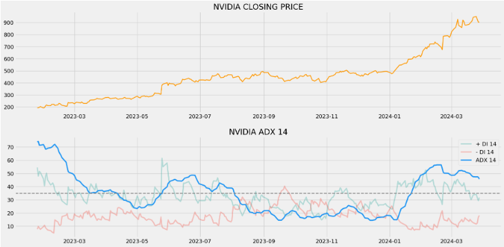
<span class="hljs-comment"># ADX PLOT</span>
plot_data = aapl[aapl.index >= <span class="hljs-string">'2023-01-03'</span>]
ax1 = plt.subplot2grid((<span class="hljs-number">11</span>,<span class="hljs-number">1</span>), (<span class="hljs-number">0</span>,<span class="hljs-number">0</span>), rowspan = <span class="hljs-number">5</span>, colspan = <span class="hljs-number">1</span>)
ax2 = plt.subplot2grid((<span class="hljs-number">11</span>,<span class="hljs-number">1</span>), (<span class="hljs-number">6</span>,<span class="hljs-number">0</span>), rowspan = <span class="hljs-number">5</span>, colspan = <span class="hljs-number">1</span>)
ax1.plot(plot_data[<span class="hljs-string">'close'</span>], linewidth = <span class="hljs-number">2</span>, color = <span class="hljs-string">'#ff9800'</span>)
ax1.set_title(<span class="hljs-string">'NVIDIA CLOSING PRICE'</span>)
ax2.plot(plot_data[<span class="hljs-string">'plus_di'</span>], color = <span class="hljs-string">'#26a69a'</span>, label = <span class="hljs-string">'+ DI 14'</span>, linewidth = <span class="hljs-number">3</span>, alpha = <span class="hljs-number">0.3</span>)
ax2.plot(plot_data[<span class="hljs-string">'minus_di'</span>], color = <span class="hljs-string">'#f44336'</span>, label = <span class="hljs-string">'- DI 14'</span>, linewidth = <span class="hljs-number">3</span>, alpha = <span class="hljs-number">0.3</span>)
ax2.plot(plot_data[<span class="hljs-string">'adx'</span>], color = <span class="hljs-string">'#2196f3'</span>, label = <span class="hljs-string">'ADX 14'</span>, linewidth = <span class="hljs-number">3</span>)
ax2.axhline(<span class="hljs-number">35</span>, color = <span class="hljs-string">'grey'</span>, linewidth = <span class="hljs-number">2</span>, linestyle = <span class="hljs-string">'--'</span>)
ax2.legend()
ax2.set_title(<span class="hljs-string">'NVIDIA ADX 14'</span>)
plt.show()</pre></div><figure id="3d67"><img src="https://cdn-images-1.readmedium.com/v2/resize:fit:800/1*LpL83nm3VrZo7TWKYE2YXA.png"><figcaption>NVIDIA Closing Price vs ADX 14 Indicator</figcaption></figure><ul><li>Step 3: RSI Calculation & Plot</li></ul><div id="c3ce"><pre><span class="hljs-comment"># RSI CALCULATION</span>
<span class="hljs-keyword">def</span> <span class="hljs-title function_">get_rsi</span>(<span class="hljs-params">close, lookback</span>):
ret = close.diff()
up = []
down = []
<span class="hljs-keyword">for</span> i <span class="hljs-keyword">in</span> <span class="hljs-built_in">range</span>(<span class="hljs-built_in">len</span>(ret)):
<span class="hljs-keyword">if</span> ret[i] < <span class="hljs-number">0</span>:
up.append(<span class="hljs-number">0</span>)
down.append(ret[i])
<span class="hljs-keyword">else</span>:
up.append(ret[i])
down.append(<span class="hljs-number">0</span>)
up_series = pd.Series(up)
down_series = pd.Series(down).<span class="hljs-built_in">abs</span>()
up_ewm = up_series.ewm(com = lookback - <span class="hljs-number">1</span>, adjust = <span class="hljs-literal">False</span>).mean()
down_ewm = down_series.ewm(com = lookback - <span class="hljs-number">1</span>, adjust = <span class="hljs-literal">False</span>).mean()
rs = up_ewm/down_ewm
rsi = <span class="hljs-number">100</span> - (<span class="hljs-number">100</span> / (<span class="hljs-number">1</span> + rs))
rsi_df = pd.DataFrame(rsi).rename(columns = {<span class="hljs-number">0</span>:<span class="hljs-string">'rsi'</span>}).set_index(close.index)
rsi_df = rsi_df.dropna()
<span class="hljs-keyword">return</span> rsi_df[<span class="hljs-number">3</span>:]
aapl[<span class="hljs-string">'rsi_14'</span>] = get_rsi(aapl[<span class="hljs-string">'close'</span>], <span class="hljs-number">14</span>)
aapl = aapl.dropna()
aapl.tail()
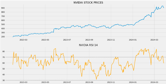
<span class="hljs-comment"># RSI PLOT</span>
plot_data = aapl[aapl.index >= <span class="hljs-string">'2023-01-03'</span>]
ax1 = plt.subplot2grid((<span class="hljs-number">11</span>,<span class="hljs-number">1</span>), (<span class="hljs-number">0</span>,<span class="hljs-number">0</span>), rowspan = <span class="hljs-number">5</span>, colspan = <span class="hljs-number">1</span>)
ax2 = plt.subplot2grid((<span class="hljs-number">11</span>,<span class="hljs-number">1</span>), (<span class="hljs-number">6</span>,<span class="hljs-number">0</span>), rowspan = <span class="hljs-number">5</span>, colspan = <span class="hljs-number">1</span>)
ax1.plot(plot_data[<span class="hljs-string">'close'</span>], linewidth = <span class="hljs-number">2.5</span>)
ax1.set_title(<span class="hljs-string">'NVIDIA STOCK PRICES'</span>)
ax2.plot(plot_data[<span class="hljs-string">'rsi_14'</span>], c
Options
olor = <span class="hljs-string">'orange'</span>, linewidth = <span class="hljs-number">2.5</span>)
ax2.axhline(<span class="hljs-number">30</span>, linestyle = <span class="hljs-string">'--'</span>, linewidth = <span class="hljs-number">1.5</span>, color = <span class="hljs-string">'grey'</span>)
ax2.axhline(<span class="hljs-number">70</span>, linestyle = <span class="hljs-string">'--'</span>, linewidth = <span class="hljs-number">1.5</span>, color = <span class="hljs-string">'grey'</span>)
ax2.set_title(<span class="hljs-string">'NVIDIA RSI 14'</span>)
plt.show()
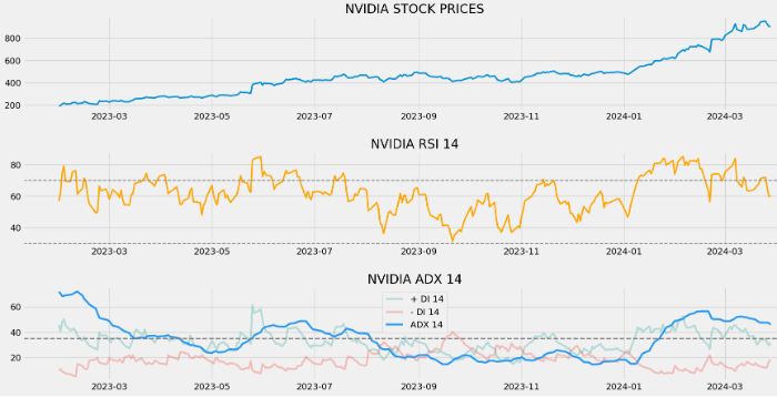
<span class="hljs-comment"># RSI ADX PLOT</span>
plot_data = aapl[aapl.index >= <span class="hljs-string">'2023-01-03'</span>]
ax1 = plt.subplot2grid((<span class="hljs-number">19</span>,<span class="hljs-number">1</span>), (<span class="hljs-number">0</span>,<span class="hljs-number">0</span>), rowspan = <span class="hljs-number">5</span>, colspan = <span class="hljs-number">1</span>)
ax2 = plt.subplot2grid((<span class="hljs-number">19</span>,<span class="hljs-number">1</span>), (<span class="hljs-number">7</span>,<span class="hljs-number">0</span>), rowspan = <span class="hljs-number">5</span>, colspan = <span class="hljs-number">1</span>)
ax3 = plt.subplot2grid((<span class="hljs-number">19</span>,<span class="hljs-number">1</span>), (<span class="hljs-number">14</span>,<span class="hljs-number">0</span>), rowspan = <span class="hljs-number">5</span>, colspan = <span class="hljs-number">1</span>)
ax1.plot(plot_data[<span class="hljs-string">'close'</span>], linewidth = <span class="hljs-number">2.5</span>)
ax1.set_title(<span class="hljs-string">'NVIDIA STOCK PRICES'</span>)
ax2.plot(plot_data[<span class="hljs-string">'rsi_14'</span>], color = <span class="hljs-string">'orange'</span>, linewidth = <span class="hljs-number">2.5</span>)
ax2.axhline(<span class="hljs-number">30</span>, linestyle = <span class="hljs-string">'--'</span>, linewidth = <span class="hljs-number">1.5</span>, color = <span class="hljs-string">'grey'</span>)
ax2.axhline(<span class="hljs-number">70</span>, linestyle = <span class="hljs-string">'--'</span>, linewidth = <span class="hljs-number">1.5</span>, color = <span class="hljs-string">'grey'</span>)
ax2.set_title(<span class="hljs-string">'NVIDIA RSI 14'</span>)
ax3.plot(plot_data[<span class="hljs-string">'plus_di'</span>], color = <span class="hljs-string">'#26a69a'</span>, label = <span class="hljs-string">'+ DI 14'</span>, linewidth = <span class="hljs-number">3</span>, alpha = <span class="hljs-number">0.3</span>)
ax3.plot(plot_data[<span class="hljs-string">'minus_di'</span>], color = <span class="hljs-string">'#f44336'</span>, label = <span class="hljs-string">'- DI 14'</span>, linewidth = <span class="hljs-number">3</span>, alpha = <span class="hljs-number">0.3</span>)
ax3.plot(plot_data[<span class="hljs-string">'adx'</span>], color = <span class="hljs-string">'#2196f3'</span>, label = <span class="hljs-string">'ADX 14'</span>, linewidth = <span class="hljs-number">3</span>)
ax3.axhline(<span class="hljs-number">35</span>, color = <span class="hljs-string">'grey'</span>, linewidth = <span class="hljs-number">2</span>, linestyle = <span class="hljs-string">'--'</span>)
ax3.legend()
ax3.set_title(<span class="hljs-string">'NVIDIA ADX 14'</span>)
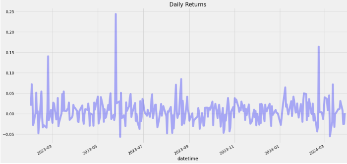
plt.show()</pre></div><figure id="0869"><img src="https://cdn-images-1.readmedium.com/v2/resize:fit:800/1*q6HOIkJOTi8mb1xVB3LMzA.png"><figcaption>NVIDIA Stock Price vs RSI 14 Indicator</figcaption></figure><figure id="7073"><img src="https://cdn-images-1.readmedium.com/v2/resize:fit:800/1*gP0q_JPQpyBCD8rQHLZFpg.png"><figcaption>NVIDIA Stock Price vs RSI & ADX 14 Indicators</figcaption></figure><ul><li>Step 4: NVIDIA Daily & Cumulative Returns</li></ul><div id="960b"><pre>rets = aapl.close.pct_change().dropna()
strat_rets = strategy.adx_rsi_position[<span class="hljs-number">1</span>:]*rets
plt.title(<span class="hljs-string">'Daily Returns'</span>)
rets.plot(color = <span class="hljs-string">'blue'</span>, alpha = <span class="hljs-number">0.3</span>, linewidth = <span class="hljs-number">7</span>)
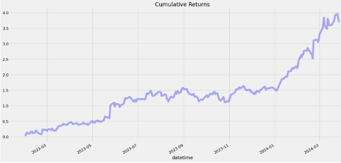
plt.show()</pre></div><figure id="972e"><img src="https://cdn-images-1.readmedium.com/v2/resize:fit:800/1*lmqcRauPPxiTMVMUNVeI7w.png"><figcaption>NVIDIA Daily Returns</figcaption></figure><div id="8ce8"><pre>rets_cum = (<span class="hljs-number">1</span> + rets).cumprod() - <span class="hljs-number">1</span>
strat_cum = (<span class="hljs-number">1</span> + strat_rets).cumprod() - <span class="hljs-number">1</span>
plt.title(<span class="hljs-string">'Cumulative Returns'</span>)
rets_cum.plot(color = <span class="hljs-string">'blue'</span>, alpha = <span class="hljs-number">0.3</span>, linewidth = <span class="hljs-number">7</span>)
plt.show()</pre></div><figure id="aa9a"><img src="https://cdn-images-1.readmedium.com/v2/resize:fit:800/1*XkOZtGWdKFM2pFOCUCzjxw.png"><figcaption>NVIDIA Cumulative Returns</figcaption></figure><h2 id="2a2a">Conclusions</h2><ul><li>The ADX values ~50+/-5 suggest a very strong trend in Q1'24. However, a decreasing ADX curve indicates that the movement is losing momentum.</li><li>High RSI levels, ~70+/-10, generate sell signals and suggest that NVIDIA is overbought or <a href="https://www.investopedia.com/terms/o/overvalued.asp">overvalued</a> in Q1'24.</li><li>The 1Y stock cumulative returns confirm a reasonable profit (excluding all costs) of the benchmark passive strategy.</li><li>The road ahead: AI-powered stock price forecasting, stochastic simulations, backtesting and benchmarking against S&P 500 in 2024.</li></ul><h2 id="5a33">Explore More</h2><ul><li><a href="https://readmedium.com/algo-trading-nvidia-with-williams-r-macd-indicators-a85dcd70c8cb">Algo-Trading NVIDIA with Williams %R & MACD Indicators</a></li><li><a href="https://readmedium.com/an-algo-trading-sneak-peek-at-top-ai-powered-growth-stocks-1-nvidia-8cbc06c0de5f">An Algo-Trading Sneak Peek at Top AI-Powered Growth Stocks — 1. NVIDIA</a></li><li><a href="https://readmedium.com/useful-fintech-saas-products-guides-blogs-for-quant-trading-b6e65b423b0b">Useful FinTech SaaS Products, Guides & Blogs for Quant Trading</a></li><li><a href="https://wp.me/pdMwZd-7dI">NVIDIA Returns-Drawdowns MVA & RNN Mean Reversal Trading</a></li><li><a href="https://wp.me/pdMwZd-7by">NVIDIA Rolling Volatility: GARCH & XGBoost</a></li><li><a href="https://wp.me/pdMwZd-71E">IQR-Based Log Price Volatility Ranking of Top 19 Blue Chips</a></li></ul><h2 id="593b">References</h2><ul><li><a href="https://readmedium.com/does-combining-adx-and-rsi-create-a-better-profitable-trading-strategy-125a90c36ac">Does Combining ADX and RSI Create a Better Profitable Trading Strategy?</a></li><li><a href="https://tradeciety.com/how-to-choose-the-best-indicators-for-your-trading">HOW TO COMBINE THE BEST INDICATORS AND AVOID WRONG SIGNALS</a></li><li><a href="https://www.tradingview.com/chart/EURUSD/iWijQ5qD-ADX-Trend-Based-Strategies/">ADX Trend-Based Strategies</a></li><li><a href="https://www.quantifiedstrategies.com/rsi-adx-trading-strategy/">RSI & ADX Trading Strategies (Backtest and Rules)</a></li><li><a href="https://www.dukascopy.com/swiss/english/marketwatch/articles/demystifying-the-relative-strength-index-(rsi)-indicator/">DEMYSTIFYING THE RELATIVE STRENGTH INDEX (RSI) INDICATOR</a></li></ul><h2 id="fa2a">Keywords</h2><ul><li>#Python</li><li>#NVDA</li><li>#AI</li><li>#algotrading</li><li>#trading</li><li>#investment</li><li>#fintech</li><li>#finance</li><li>#stockmarket</li><li>#stocks</li></ul><h2 id="9de6">Contacts</h2><ul><li><a href="https://wp.me/PdMwZd-3nr">Website</a></li><li><a href="https://twitter.com/alzapress">Twitter</a></li><li><a href="https://nl.pinterest.com/alexzap922/">Pinterest</a></li></ul></article></body>