Portfolio Optimization (PO) of 25 Largest US Tech Stocks: A Four-Fold Risk/Return Analysis

Comparing Riskfolio-Lib Mean Risk PO to Max Sharpe Monte Carlo Simulations, SciPy SLSQP Minimization, and Pyfolio Rebalancing of 25 Largest US Tech Stocks vs S&P 500 Benchmark

In investing, PO is the task of selecting assets such that the return on investment is maximized while the risk is minimized [1–4].
Finding the right methods for PO [1–4] (mean-variance optimization, Monte Carlo simulations, risk parity, least squares optimization, etc.) is an important part of the work done by investment banks and asset management firms.
Here, we will look at how to apply these methods to construct an optimal portfolio of stocks within the tech industry.
Our goal is to explore the essential Python tools and libraries for PO, walk through the process of calculating fundamental portfolio metrics, and outline how proven PO strategies can be applied in practice.
Why use Python for PO:

Python provides a great collection of specialized fintech packages, tools and APIs suitable for financial markets.

Assets:

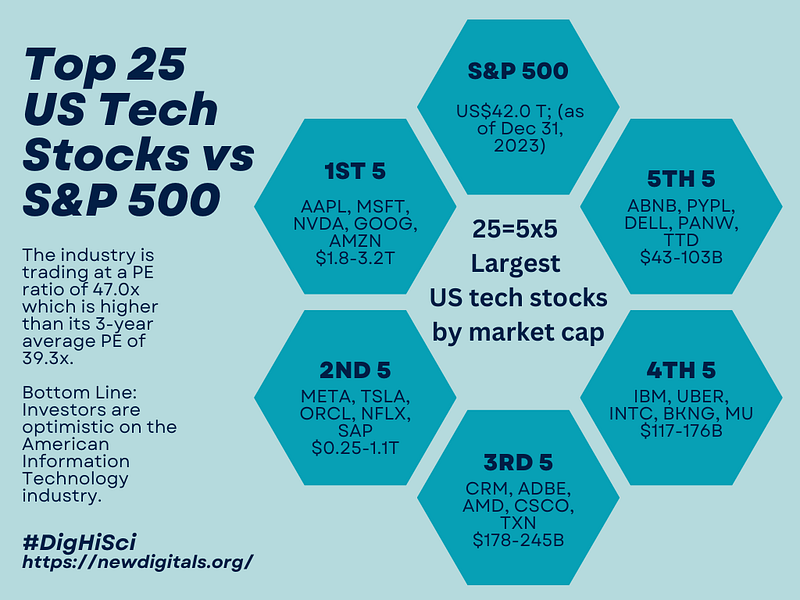
Our investment portfolio consists of 25 Largest US Tech Stocks by market cap

# Tickers of assets
assets = ['DELL', 'ABNB', 'PANW', 'BKNG', 'UBER', 'IBM', 'SCCO', 'ADBE',
          'NFLX', 'SAP', 'TXN', 'ORCL', 'TTD', 'MU', 'PYPL', 'INTC',
          'GOOG', 'MSFT', 'NVDA', 'AMZN', 'META', 'TSLA', 'AAPL', 'AMD', 'CRM']

len(assets)
25

# Date range
start = '2020-01-01'
end = '2024-07-26'

Tools:

Riskfolio-Lib is a library for making quantitative strategic asset allocation or portfolio optimization in Python. It is built on top of cvxpy and closely integrated with pandas data structures.
The SciPy minimize(method=’SLSQP’) minimizes a scalar function of several variables using Sequential Least Squares Programming (SLSQP).
MPT PO is based on Monte Carlo Simulations for Optimization Search of max Sharpe ratio for a given level of market risk, emphasizing that risk is an inherent part of higher reward.
Portfolio rebalancing is a technique that involves adjusting the asset allocation dynamically to keep it in line with investment goals.
pyfolio is a Python library for performance and risk analysis of financial portfolios developed by Quantopian Inc. It works well with the Zipline open source backtesting library.

The paper is organized as follows:

Riskfolio-Lib Mean Risk Optimization Algorithms
MPT Random Search of max Sharpe Ratio Portfolio
SciPy SLSQP Numerical Optimization Strategy
Portfolio Rebalancing Strategy
Pyfolio Backtesting Analysis

Riskfolio-Lib Mean Risk Optimization Algorithms

Let’s implement the Classic Mean Risk PO [1] using Riskfolio-Lib.
Reading the input stock data and calculating their daily returns

import numpy as np
import pandas as pd
import yfinance as yf
import warnings

warnings.filterwarnings("ignore")
pd.options.display.float_format = '{:.4%}'.format

# Downloading data
data = yf.download(assets, start = start, end = end)
data = data.loc[:,('Adj Close', slice(None))]
data.columns = assets

# Calculating returns

Y = data[assets].pct_change().dropna()

Estimating mean variance portfolios

import riskfolio as rp

# Building the portfolio object
port = rp.Portfolio(returns=Y)

# Calculating optimal portfolio

# Select method and estimate input parameters:

method_mu='hist' # Method to estimate expected returns based on historical data.
method_cov='hist' # Method to estimate covariance matrix based on historical data.

port.assets_stats(method_mu=method_mu, method_cov=method_cov)

# Estimate optimal portfolio:

model='Classic' # Could be Classic (historical), BL (Black Litterman) or FM (Factor Model)
rm = 'MV' # Risk measure used, this time will be variance
obj = 'Sharpe' # Objective function, could be MinRisk, MaxRet, Utility or Sharpe
hist = True # Use historical scenarios for risk measures that depend on scenarios
rf = 0 # Risk free rate
l = 0 # Risk aversion factor, only useful when obj is 'Utility'

w = port.optimization(model=model, rm=rm, obj=obj, rf=rf, l=l, hist=hist)

# Plotting the composition of the portfolio

ax = rp.plot_pie(w=w, title='Sharpe Mean Variance', others=0.05, nrow=25, cmap = "tab20",
                 height=6, width=10, ax=None)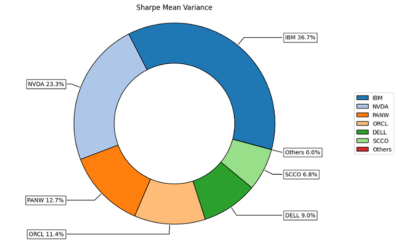

Composition of the Sharpe Mean Variance Portfolio

Calculating and plotting the MPT efficient frontier

#Calculate efficient frontier
points = 100 # Number of points of the frontier

frontier = port.efficient_frontier(model=model, rm=rm, points=points, rf=rf, hist=hist)

# Plotting the efficient frontier

label = 'Max Risk Adjusted Return Portfolio' # Title of point
mu = port.mu # Expected returns
cov = port.cov # Covariance matrix
returns = port.returns # Returns of the assets

ax = rp.plot_frontier(w_frontier=frontier, mu=mu, cov=cov, returns=returns, rm=rm,
                      rf=rf, alpha=0.05, cmap='viridis', w=w, label=label,
                      marker='*', s=16, c='r', height=6, width=10, ax=None)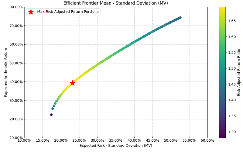

Plotting the efficient frontier’s asset structure

# Plotting the efficient frontier composition

ax = rp.plot_frontier_area(w_frontier=frontier, cmap="tab20", height=6, width=10, ax=None)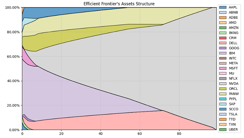

Calculating the optimal portfolio that maximizes Return/CVaR ratio

#Calculating the portfolio that maximizes Return/CVaR ratio.
rm = 'CVaR' # Risk measure

w = port.optimization(model=model, rm=rm, obj=obj, rf=rf, l=l, hist=hist)

# Plotting the composition of the portfolio

ax = rp.plot_pie(w=w, title='Sharpe Mean CVaR', others=0.05, nrow=25, cmap = "tab20",
                 height=6, width=10, ax=None)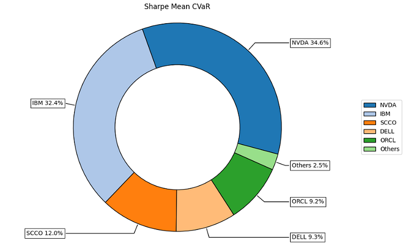

Plotting the Mean CVaR efficient frontier

points = 100 # Number of points of the frontier

frontier = port.efficient_frontier(model=model, rm=rm, points=points, rf=rf, hist=hist)

label = 'Max Risk Adjusted Return Portfolio' # Title of point

ax = rp.plot_frontier(w_frontier=frontier, mu=mu, cov=cov, returns=returns, rm=rm,
                      rf=rf, alpha=0.05, cmap='viridis', w=w, label=label,
                      marker='*', s=16, c='r', height=6, width=10, ax=None)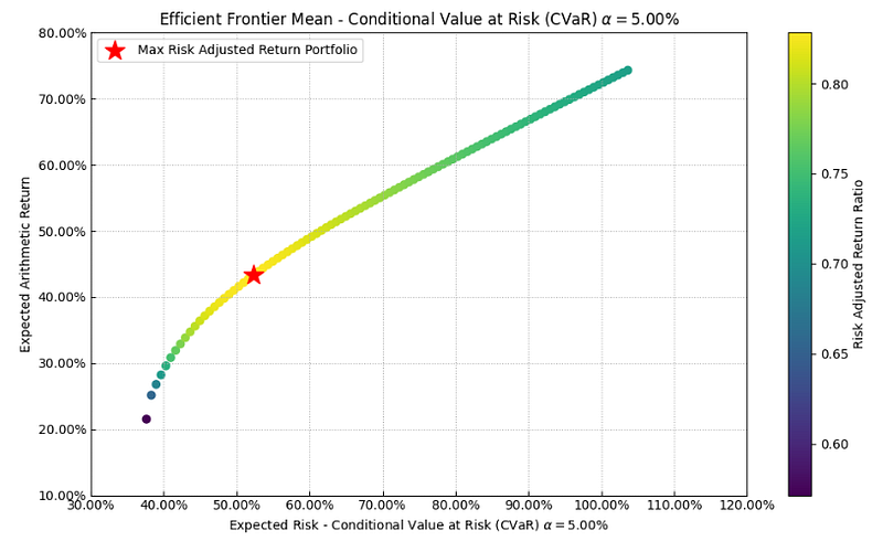

Mean CVaR Efficient Frontier & Max Risk Adjusted Return Portfolio

Plotting the Mean CVaR efficient frontier’s assets structure

# Plotting the efficient frontier composition

ax = rp.plot_frontier_area(w_frontier=frontier, cmap="tab20", height=6, width=10, ax=None)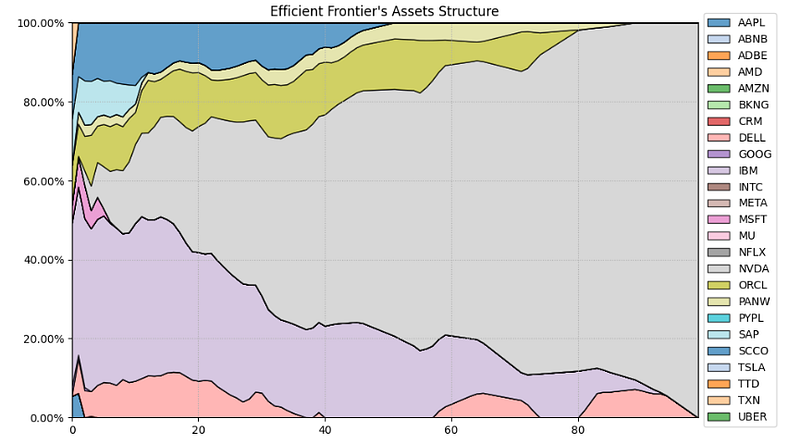

Mean CVaR Efficient Frontier’s Assets Structure

Calculating optimal portfolios for different risk measures

#Calculate Optimal Portfolios for Several Risk Measures
# Risk Measures available:
#
# 'MV': Standard Deviation.
# 'MAD': Mean Absolute Deviation.
# 'MSV': Semi Standard Deviation.
# 'FLPM': First Lower Partial Moment (Omega Ratio).
# 'SLPM': Second Lower Partial Moment (Sortino Ratio).
# 'CVaR': Conditional Value at Risk.
# 'EVaR': Entropic Value at Risk.
# 'WR': Worst Realization (Minimax)
# 'MDD': Maximum Drawdown of uncompounded cumulative returns (Calmar Ratio).
# 'ADD': Average Drawdown of uncompounded cumulative returns.
# 'CDaR': Conditional Drawdown at Risk of uncompounded cumulative returns.
# 'EDaR': Entropic Drawdown at Risk of uncompounded cumulative returns.
# 'UCI': Ulcer Index of uncompounded cumulative returns.

rms = ['MV', 'MAD', 'MSV', 'FLPM', 'SLPM', 'CVaR',
       'EVaR', 'WR', 'MDD', 'ADD', 'CDaR', 'UCI', 'EDaR']

w_s = pd.DataFrame([])

for i in rms:
    w = port.optimization(model=model, rm=i, obj=obj, rf=rf, l=l, hist=hist)
    w_s = pd.concat([w_s, w], axis=1)
    
w_s.columns = rms

w_s.style.format("{:.2%}").background_gradient(cmap='YlGn')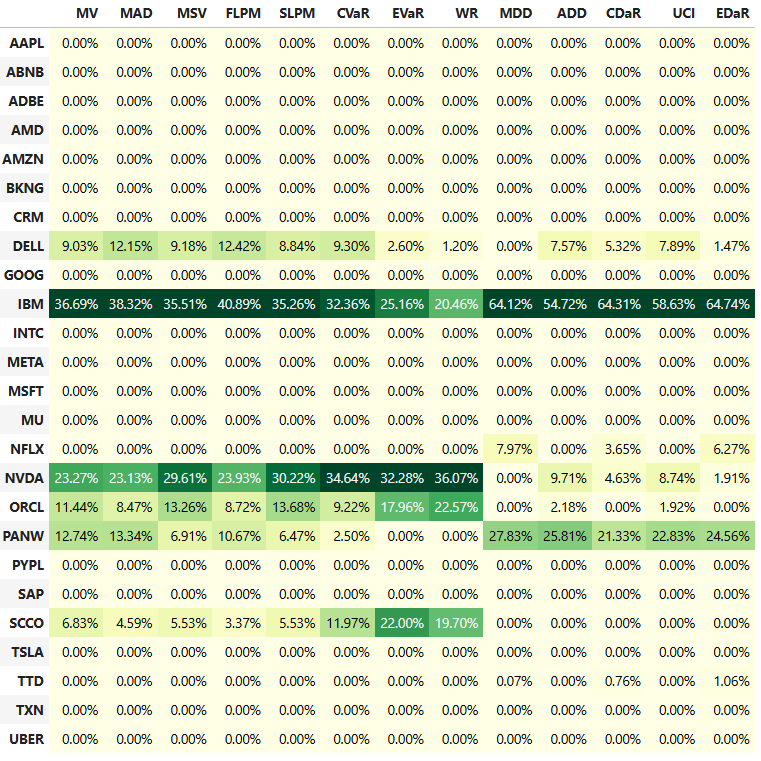

Comparing optimal portfolios for different risk measures

Comparing asset allocation weights for different risk measures

import matplotlib.pyplot as plt

# Plotting a comparison of assets weights for each portfolio

fig = plt.gcf()
fig.set_figwidth(14)
fig.set_figheight(6)
ax = fig.subplots(nrows=1, ncols=1)

w_s.plot.bar(ax=ax)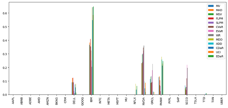

Comparing asset allocation weights for different risk measures

MPT Random Search of max Sharpe Ratio Portfolio

Implementing a random search of max Sharpe ratio [2]

import numpy as np
import pandas as pd
import matplotlib.pyplot as plt
import quandl
%matplotlib inline

#Optimization method - Randomization
df=data.copy()
print('The stocks are: ',df.columns)
np.random.seed(200)
weights = np.array(np.random.random(len(assets)))
weights = weights/np.sum(weights)
print('Random weights: ',weights)

The stocks are:  Index(['AAPL', 'ABNB', 'ADBE', 'AMD', 'AMZN', 'BKNG', 'CRM', 'DELL', 'GOOG',
       'IBM', 'INTC', 'META', 'MSFT', 'MU', 'NFLX', 'NVDA', 'ORCL', 'PANW',
       'PYPL', 'SAP', 'SCCO', 'TSLA', 'TTD', 'TXN', 'UBER'],
      dtype='object')
Random weights:  [0.06301366 0.01506448 0.03952651 0.02848077 0.05081223 0.00019022
 0.02376721 0.06049098 0.03032752 0.06528586 0.05767569 0.06556679
 0.06139346 0.02019436 0.05626242 0.00806076 0.05223761 0.01665756
 0.00638558 0.06273829 0.05492895 0.0344665  0.0580842  0.03845962
 0.02992878]

Calculating the asset log daily returns, covariance, expected annual return/volatility, and Sharpe ratio

log_returns = np.log(df/df.shift(1))
log_returns.cov()

expected_return = np.sum((log_returns.mean()* weights) * 252)
expected_return
0.1802899466955814

expected_vol = np.sqrt(np.dot(weights.T,np.dot(log_returns.cov()*252,weights)))
expected_vol
0.28410143028979384

sharpe_r = expected_return/expected_vol
sharpe_r
0.6345971103055661

Finding max Sharpe ratio

np.random.seed(200)

# Initalization of variables
portfolio_number = 10000
weights_total = np.zeros((portfolio_number,len(df.columns)))
returns = np.zeros(portfolio_number)
volatility = np.zeros(portfolio_number)
sharpe = np.zeros(portfolio_number)

for i in range(portfolio_number):

    # Random weights
    weights = np.array(np.random.random(len(assets)))
    weights = weights/np.sum(weights)
    # Append weight
    weights_total[i,:] = weights

    # Expected return
    returns[i] = np.sum((log_returns.mean()* weights) * 252)

    # Expected volume
    volatility[i] = np.sqrt(np.dot(weights.T,np.dot(log_returns.cov()*252,weights)))

    # Sharpe ratio
    sharpe[i] = returns[i]/volatility[i]

max_sharpe = sharpe.max()
max_sharpe
0.8079766401400306

max_sharpe_index = sharpe.argmax()
max_sharpe_index
6117

max_sharpe_weights = weights_total[6117,:]
max_sharpe_weights

array([0.03369816, 0.02384189, 0.03073916, 0.01557581, 0.02691991,
       0.01677664, 0.01131073, 0.07801402, 0.02552391, 0.08765475,
       0.00925351, 0.0668527 , 0.08848405, 0.02780067, 0.03185717,
       0.05520476, 0.08137229, 0.00877285, 0.0032981 , 0.01804487,
       0.05128246, 0.08892774, 0.02873561, 0.07454356, 0.01551469])

max_sharpe_return = returns[max_sharpe_index]
max_sharpe_return
0.23180409433187227

max_sharpe_vol = volatility[max_sharpe_index]
max_sharpe_vol
0.28689454968858785

plt.figure(figsize=(12,8))
plt.scatter(volatility,returns,c=sharpe)
plt.colorbar(label='Sharpe Ratio')
plt.xlabel('Volatility')
plt.ylabel('Return')
plt.grid()
plt.scatter(max_sharpe_vol,max_sharpe_return,c='red',s=50)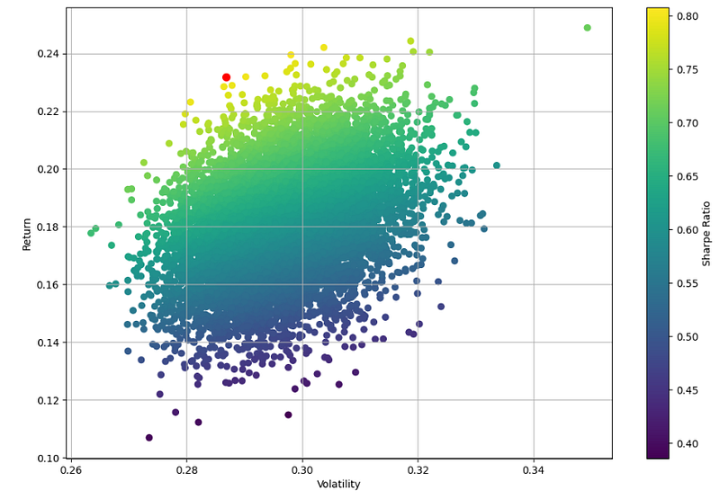

Random search of the Max Sharpe ratio portfolio

SciPy SLSQP Numerical Optimization Strategy

The SciPy module minimize can be used to find a minimum of the negative Sharpe ratio with constraints and bounds [2]

from scipy.optimize import minimize

def stats(weights):
    weights = np.array(weights)
    expected_return = np.sum((log_returns.mean()* weights) * 252)
    expected_vol = np.sqrt(np.dot(weights.T,np.dot(log_returns.cov()*252,weights)))
    sharpe_r = expected_return/expected_vol
    return np.array([expected_return,expected_vol,sharpe_r])

def sr_negate(weights):
    neg_sr = stats(weights)[2] * -1
    return neg_sr

def weight_check(weights):
    weights_sum = np.sum(weights)
    return weights_sum - 1

constraints = ({'type':'eq','fun':weight_check})
bounds = ((0,1),(0,1),(0,1),(0,1),(0,1),(0,1),(0,1),(0,1),(0,1),(0,1),(0,1),(0,1),(0,1),
          (0,1),(0,1),(0,1),(0,1),(0,1),(0,1),(0,1),(0,1),(0,1),(0,1),(0,1),(0,1))
initial_guess = [0.06301366, 0.01506448, 0.03952651, 0.02848077, 0.05081223, 0.00019022,
 0.02376721, 0.06049098, 0.03032752, 0.06528586, 0.05767569, 0.06556679,
 0.06139346, 0.02019436, 0.05626242, 0.00806076, 0.05223761, 0.01665756,
 0.00638558, 0.06273829, 0.05492895, 0.0344665,  0.0580842,  0.03845962,
 0.02992878]

len(bounds)
25

results = minimize(sr_negate,initial_guess,method='SLSQP',bounds=bounds,constraints=constraints)
results

message: Optimization terminated successfully
 success: True
  status: 0
     fun: -1.2355832799875217
       x: [ 3.456e-16  9.365e-17 ...  0.000e+00  0.000e+00]
     nit: 10
     jac: [ 9.174e-02  7.627e-01 ...  3.945e-01  4.567e-01]
    nfev: 261
    njev: 10

wt = results.x
wt
array([3.45596111e-16, 9.36519265e-17, 2.87335822e-16, 5.54679980e-16,
       0.00000000e+00, 0.00000000e+00, 0.00000000e+00, 1.22592595e-01,
       9.67429272e-18, 2.76095894e-02, 1.13175203e-15, 6.27582963e-17,
       0.00000000e+00, 1.69816242e-16, 1.56653996e-17, 5.61151766e-01,
       8.63134912e-02, 9.11149262e-02, 0.00000000e+00, 4.67141979e-17,
       8.80610161e-02, 2.31566162e-02, 1.55212414e-16, 0.00000000e+00,
       0.00000000e+00])

stats(wt)
array([0.48484961, 0.39240545, 1.23558328])

Plotting the efficient frontier, expected and max Sharpe ratio

#Plot efficient frontier
frontier_return = np.linspace(-0.6,0.4,200)

def min_vol(weights):
    vol = stats(weights)[1]
    return vol

frontier_volatility = []

for exp_return in frontier_return:
    constraints = ({'type':'eq','fun':weight_check},
                   {'type':'eq','fun':lambda x: stats(x)[0]-exp_return})
    result = minimize(min_vol,initial_guess,method='SLSQP',bounds=bounds,constraints=constraints)
    frontier_volatility.append(result['fun'])

plt.figure(figsize=(12,8))
plt.scatter(volatility,returns,c=sharpe)
plt.scatter(max_sharpe_vol,max_sharpe_return,c='red',s=200)
plt.scatter(expected_vol,expected_return,c='black',s=200)
plt.colorbar(label='Sharpe Ratio')
plt.xlabel('Volatility')
plt.ylabel('Return')
plt.ylim((0, 0.45))
plt.plot(frontier_volatility,frontier_return,'r--',linewidth=3)
plt.grid()
plt.legend(['Optimizer', 'Max Sharpe Ratio','Expected Sharpe Ratio','Frontier Line'])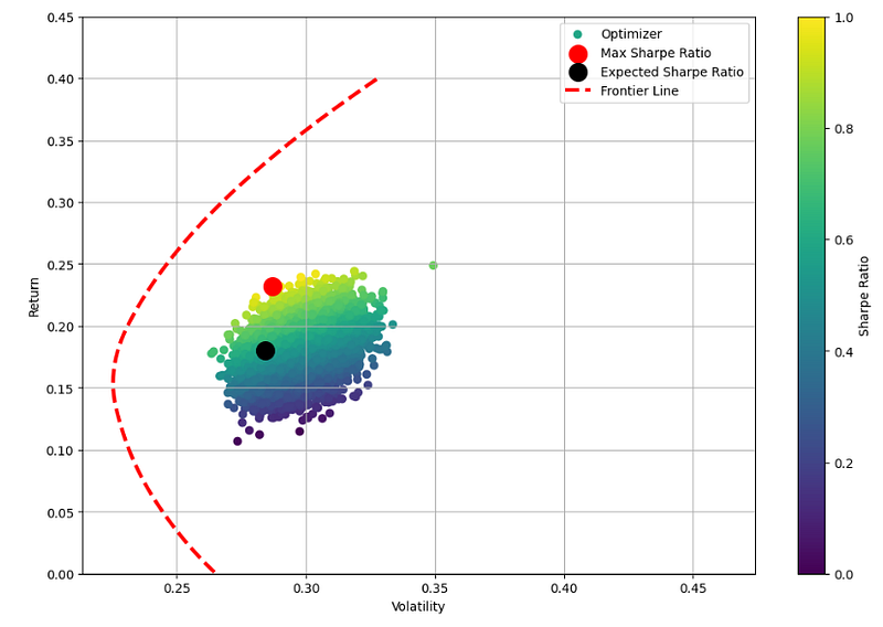

The above max and expected Sharpe ratio portfolios lie below the efficient frontier. These portfolios are sub-optimal because they do not provide enough return for the level of risk.

Portfolio Rebalancing Strategy

Implementing the following three-step portfolio rebalancing strategy [3]:

Define the assets, weights, benchmark, the initial capital, and dates;
Implement the rebalancing engine based on monthly, yearly, daily, or signal-based triggers.
Monitor the portfolio’s performance and get inferences.

Implementing step 1

# Selecting libraries
import yfinance as yf
import pandas as pd
import numpy as np
import pyfolio as py
import plotly.graph_objs as go
from plotly.subplots import make_subplots
import warnings
warnings.filterwarnings("ignore")

# User inputs
stocks = assets  # Assets to select yfinance format
portfolio_value = 10**6                        # Initial portfolio value to be allocated
weights = [0.06301366, 0.01506448, 0.03952651, 0.02848077, 0.05081223, 0.00019022,
 0.02376721, 0.06049098, 0.03032752, 0.06528586, 0.05767569, 0.06556679,
 0.06139346, 0.02019436, 0.05626242, 0.00806076, 0.05223761, 0.01665756,
 0.00638558, 0.06273829, 0.05492895, 0.0344665,  0.0580842,  0.03845962,
 0.02992878]    # Weight allocation per asset

benchmark = '^GSPC' # Which is your benchmark? 

start_date = '2020-01-01'   # Start date for asset data download
live_date = '2024-07-26'    # Portfolio LIVE start date (for analytics)

#Reading input data

stock_data = yf.download(stocks, start=start_date)['Adj Close']
stock_data = stock_data.dropna()
stock_data = stock_data.reindex(columns=stocks) #! Key to mantain structure
stock_prices = stock_data[stocks].values

shares_df = pd.DataFrame(index=[stock_data.index[0]])

for s,w in zip(stocks, weights):
    shares_df[s + '_shares'] = np.floor((portfolio_value * np.array(w)) / stock_data[s][0])

Implementing step 2

# REBALANCING ENGINE (change between .year, .month, .day to execute the rebalancing

# initialize variables
balance_year = stock_data.index[0].year # Since we rebalance based on year
signal = False 
count = 0    # for loop count purpose

# Store previous values in a dictionary
prev_values = {}

# Calculate portfolio value for the first day by mult. shares * price per asset at t=0
portfolio_value = sum([shares_df.loc[stock_data.index[0], s + '_shares'] * stock_data.loc[stock_data.index[0], s] for s in stocks])

for day in stock_data.index:
    count += 1
    if day == stock_data.index[0]:
        shares_df.loc[day] = shares_df.loc[day] # First day
        # Store initial values as previous values
        for col in shares_df.columns:
            prev_values[col] = shares_df.loc[day, col]

    elif day.year != balance_year: # THIS IS OUR SIGNAL
        signal = True
        # calculate new shares based on the new portfolio value and weights
        new_shares = [np.floor((portfolio_value * w) / stock_data[s][day]) for s,w in zip(stocks, weights)]
        shares_df.loc[day, :] = new_shares
        balance_year = day.year
        count += 1
        # print(f'Rebalance: {day.date()}, count: {count}') # uncomment to debug days ;)
        # Store new values as previous values
        for col in shares_df.columns:
            prev_values[col] = shares_df.loc[day, col]

    else:
        signal = False
        # Use previous values if it is not a rebalancing date
        shares_df.loc[day, :] = [prev_values[col] for col in shares_df.columns]
        # print(f'Not rebalance, regular day: {day.date()}') # uncomment to debug days ;)

    # Calculate asset values and portfolio value for the current day
    asset_values = [shares_df.loc[day, s + '_shares'] * stock_data.loc[day, s] for s in stocks]
    portfolio_value = sum(asset_values)
    stock_data.loc[day, 'Signal'] = signal
    stock_data.loc[day, 'Portfolio_Value'] = portfolio_value
    
    # Add shares to stock data frame to have all together
    for s in stocks:
        stock_data.loc[day, s + '_shares'] = shares_df.loc[day, s + '_shares']
        stock_data.loc[day, s + '_value'] = shares_df.loc[day, s + '_shares'] * stock_data.loc[day, s]

Pyfolio Backtesting Analysis

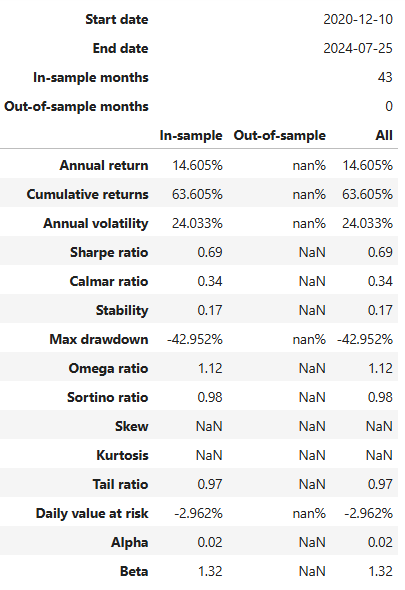
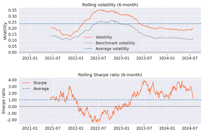
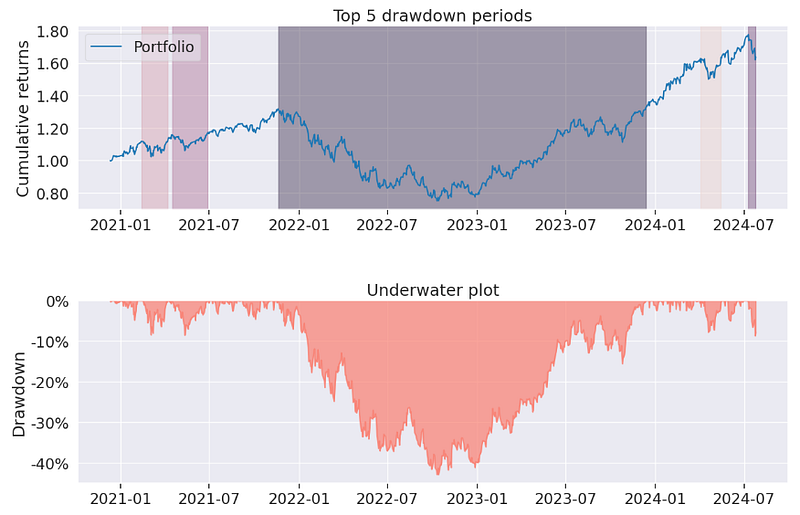
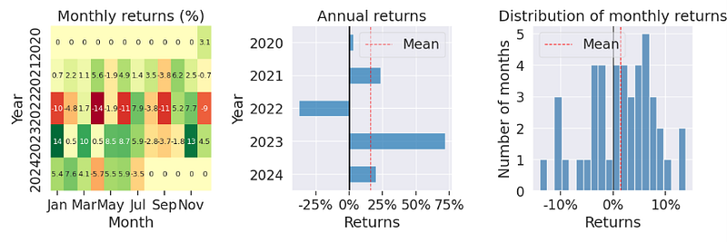
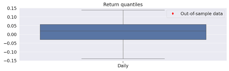
Implementing step 3 with pyfolio backtesting vs S&P 500 benchmark [3]

# Calculate log returns for portfolio
stock_data['Portfolio_Value_rets'] = np.log(stock_data['Portfolio_Value'] / stock_data['Portfolio_Value'].shift(1))

# Calculate log returns for each stock and asset weight
for stock in stocks:
    stock_data[f'{stock}_rets'] = np.log(stock_data[stock] / stock_data[stock].shift(1))
    stock_data[stock + '_weight'] = stock_data[stock + '_value'] / stock_data['Portfolio_Value']

# Benchmark data download and return
start_date_benchmark = stock_data.index[0]
benchmark_data = yf.download(benchmark, start=start_date_benchmark)
benchmark_data = benchmark_data.dropna()
benchmark_data['benchmark_rets'] = np.log(benchmark_data['Adj Close'] / benchmark_data['Adj Close'].shift(1))
benchmark_data['benchmark_rets'] = benchmark_data['benchmark_rets'].dropna()

# Data timezone unification for pyfolio valuation
#stock_data.index = stock_data.index.tz_localize('UTC')
#benchmark_data.index = benchmark_data.index.tz_localize('UTC')

stock_data.index = stock_data.index.tz_localize('UTC')
benchmark_data.index = benchmark_data.index.tz_localize('UTC')

live_date = pd.Timestamp(live_date, tz='UTC')

from IPython.core.display import display, HTML
display(HTML("<style>div.output_scroll { height: 44em; }</style>"))
py.create_full_tear_sheet(stock_data['Portfolio_Value_rets'], benchmark_rets = benchmark_data['benchmark_rets'], live_start_date = live_date)

Portfolio Value Evaluation: Worst drawdown periods & stress events

Cumulative Returns: Backtest vs Benchmark

Cumulative Returns volatility matched benchmark vs log scale.

Portfolio Daily Returns & Rolling portfolio/benchmark beta

Top 5 drawdown periods vs underwater plot

Monthly, annual returns and distribution of monthly returns

Conclusions

The Riskfolio-Lib Sharpe Mean Variance portfolio

Return ~ 40%, Risk ~ 23%, Risk Adjusted Sharpe Ratio ~ 1.7

Top 2 assets: NVDA (23%), IBM (37%)

The Riskfolio-Lib Mean CVaR portfolio

Return ~ 42%, Risk ~ 52%, Risk Adjusted Sharpe Ratio ~ 0.83

Top 2 assets: NVDA (35%), IBM (32%)

Riskfolio-Lib optimal portfolios for different risk measures

Top_Assets Risk_Metrics Max_Return %
IBM        EDaR          65
NVDA       WR            36
ORCL       WR            23
PANW       MDD           28
SCCO       EVaR          22

MPT Monte Carlo Simulation of max Sharpe Ratio Portfolio

Return ~ 23%, Risk ~ 29%, Risk Adjusted Sharpe Ratio ~ 0.81

SciPy SLSQP Numerical Optimization Strategy — suboptimal portfolio

Return ~ 23%, Risk ~ 28%, Risk Adjusted Sharpe Ratio ~ 1.0

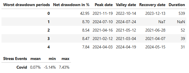
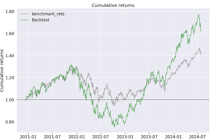
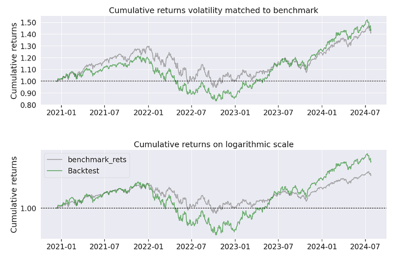
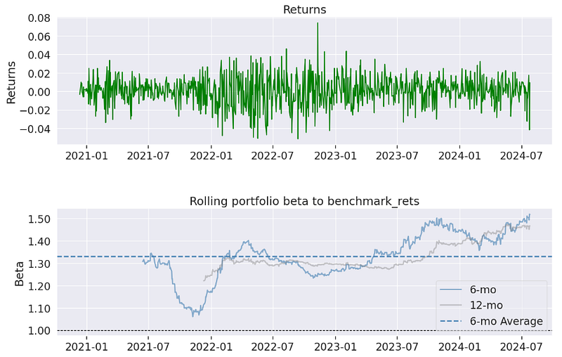
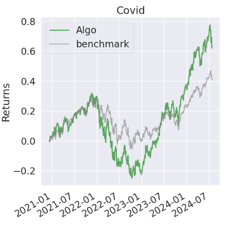
Rebalancing Strategy — Pyfolio In-Sample Backtesting Report

Annual return ~ 14.6%, annual volatility ~ 24%, cumulative return ~ 63.6%,

Sharpe ratio ~ 0.69, Calmar ratio ~ 0.34, Omega ratio ~ 1.12, Sortino ratio ~ 0.98, Alpha ~ 0.02, Beta ~ 1.32, Max drawdown ~ -43%, Daily VaR ~ -2.9%

Our ongoing work aims at evaluating the Risk Parity approach [4], harnessing the power of diversified risk rather than diversified assets.

References

Explore More

Contacts

Disclaimer

The following disclaimer clarifies that the information provided in this article is for educational use only and should not be considered financial or investment advice.
The information provided does not take into account your individual financial situation, objectives, or risk tolerance.
Any investment decisions or actions you undertake are solely your responsibility.
You should independently evaluate the suitability of any investment based on your financial objectives, risk tolerance, and investment timeframe.
It is recommended to seek advice from a certified financial professional who can provide personalized guidance tailored to your specific needs.
The tools, data, content, and information offered are impersonal and not customized to meet the investment needs of any individual. As such, the tools, data, content, and information are provided solely for informational and educational purposes only.