1Y 5 Asset Portfolio Optimization with PyPortfolioOpt: Min Volatility vs Optimal Risky Models

Image design template by @esseglo via Canva.

In algo-trading, Portfolio Optimization (PO) methods [1–5] aim to pick and size positions in financial instruments that achieve the desired risk-return trade-off regarding a benchmark.
The objective of this post is to evaluate the PO algorithm [3] that implements the PyPortfolioOpt efficient frontier or mean-variance optimization (MVO) techniques for calculating the expected returns and covariance matrix from historical stock data.
Conventionally, MVO requires knowledge of the expected returns and a risk model.
The expected_returns MVO module provides functions for estimating the expected returns of the assets. By convention, the output of these methods is expected annual returns. It is assumed that daily prices are provided.
The most commonly-used MVO risk model is the covariance matrix, which describes asset volatilities and their co-dependence.
As a quick example, we’ll optimize a diversified 1Y portfolio of the following 5 US stocks: XOM, LMT, AAPL , LYTS, and VRTX representing energy, aerospace/defense, BigTech, manufactures, and biotech sectors, respectively.

Let’s delve into the specifics of the proposed PO strategy.

Basic Imports & Installations

Setting the working directory YOURPATH

import os
os.chdir('YOURPATH')    # Set working directory
os. getcwd()

Installing Python libraries with pip

!pip install yfinance, pyportfolioopt

Importing Python libraries/modules

import pandas as pd
import numpy as np
from datetime import datetime
import matplotlib.pyplot as plt
plt.style.use("fivethirtyeight")
from pypfopt.efficient_frontier import EfficientFrontier
from pypfopt import risk_models
from pypfopt import expected_returns
from pandas_datareader import data as pdr
import yfinance as yfin
yfin.pdr_override()

Input Historical Stock Data

Defining the stock tickers and the time period

#get the stock symbols in the portfolio
assets = ["XOM", "LMT", "AAPL" , "LYTS", "VRTX"]
weights = np.array([0.2,0.2,0.2,0.2,0.2])
start='2022-01-03'
end='2023-03-10'

Fetching the Adj Close price of the above stocks

#create a dataframe to store the adjusted close proce of the stocks
df = pd.DataFrame()

#Store the adjusted close price of the stock into the df
for stock in assets:
    df[stock] = pdr.get_data_yahoo(stock, start =start, end=end)["Adj Close"]
df.tail()
           XOM        LMT        AAPL       LYTS   VRTX
Date     
2023-03-03 112.809998 477.890015 151.029999 15.10 290.510010
2023-03-06 113.809998 480.170013 153.830002 15.00 291.619995
2023-03-07 111.610001 478.660004 151.600006 15.04 286.579987
2023-03-08 109.980003 479.500000 152.869995 15.20 285.179993
2023-03-09 109.129997 475.850006 150.589996 15.88 286.880005

Plotting the Adj Close Price History

plt.figure(figsize=(12,6))
title = "Portfolio Adj. Close Price History"

my_stocks = df

#create and pllot the graph
for c in my_stocks.columns.values:
    plt.plot(my_stocks[c], label = c)

plt.title(title)
plt.xlabel("Date", fontsize =18)
plt.ylabel("Adj Price USD($)", fontsize=18)
plt.legend(my_stocks.columns.values , loc = "upper left")
plt.show()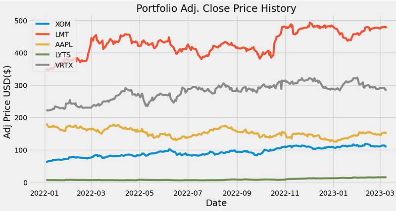

Simple Annual Portfolio Volatility vs Returns

Calculating the daily return

returns = df.pct_change()
returns

           XOM       LMT      AAPL      LYTS      VRTX
Date     
2022-01-03  NaN      NaN      NaN       NaN       NaN
2022-01-04 0.037614 0.021532 -0.012692 0.005806 -0.003011
2022-01-05 0.012437 -0.010636 -0.026600 -0.014430 -0.001983
2022-01-06 0.023521 -0.000391 -0.016693 -0.026354 0.001039
2022-01-07 0.008197 0.005978 0.000988 0.000000 0.000902
... ... ... ... ... ...
2023-03-03 0.012657 -0.000878 0.035090 0.010710 -0.000860
2023-03-06 0.008864 0.004771 0.018539 -0.006623 0.003821
2023-03-07 -0.019330 -0.003145 -0.014496 0.002667 -0.017283
2023-03-08 -0.014604 0.001755 0.008377 0.010638 -0.004885
2023-03-09 -0.007729 -0.007612 -0.014915 0.044737 0.005961
297 rows × 5 columns

Creating the annualized covariance matrix

cov_matrix_annual = returns.cov() * 252
cov_matrix_annual

    XOM      LMT       AAPL     LYTS     VRTX
XOM 0.114765 0.029406 0.031630 0.023136 0.022189
LMT 0.029406 0.063479 0.018394 -0.000315 0.016949
AAPL 0.031630 0.018394 0.118594 0.030997 0.046592
LYTS 0.023136 -0.000315 0.030997 0.262411 0.013499
VRTX 0.022189 0.016949 0.046592 0.013499 0.094169

Computing the portfolio variance as the dot product of (uniform) weights and the above matrix

port_variance = np.dot(weights.T, np.dot(cov_matrix_annual, weights))
port_variance
0.044734897834191295

Calculating the portfolio volatility aka standard deviation (std)

port_volatility = np.sqrt(port_variance)
port_volatility
0.21150625956266944

Calculating the annual portfolio return

portfolioSimpleAnnualReturn = np.sum(returns.mean()* weights)*252
portfolioSimpleAnnualReturn
0.37951677200034234

Printing the the expected annual return, volatility (risk), and variance

percent_var = str(round(port_variance,2)*100) + "%"
percent_vols = str(round(port_volatility,2)*100) + "%"
percent_ret = str(round(portfolioSimpleAnnualReturn,2)*100) + "%"

print("Expected annual return:" + percent_ret)
print("Annual volatility/risk:" + percent_vols)
print("Annual variance:" + percent_var)

Expected annual return:38.0%
Annual volatility/risk:21.0%
Annual variance:4.0%

The Efficient Frontier Optimal Portfolio: Min Volatility vs Max Sharpe Ratio

Calculating the expected returns the annualized sample covariance matrix of asset returns

mu = expected_returns.mean_historical_return(df)
S = risk_models.sample_cov(df)

#optimize for max sharpe ratio
ef = EfficientFrontier(mu , S)
weights = ef.max_sharpe()
cleaned_weights = ef.clean_weights()
print(cleaned_weights)
ef.portfolio_performance(verbose= True)

OrderedDict([('XOM', 0.36259), ('LMT', 0.26129), ('AAPL', 0.0), ('LYTS', 0.34074), ('VRTX', 0.03539)])
Expected annual return: 69.8%
Annual volatility: 25.0%
Sharpe Ratio: 2.71
(0.6975504213382199, 0.24989435276114166, 2.711347470848402)

Plotting the cumulative returns (%) of our assets

(df / df.iloc[0]*100).plot(figsize=(10,5))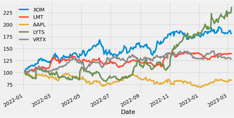

Performing 1k random simulations of portfolio returns vs volatilities

log_returns = np.log(df/df.shift(1))

portfolio_returns = []
portfolio_volatilities = []
for x in range(1000):
    weights = np.random.random(len(assets))
    weights /= np.sum(weights)
    
    portfolio_returns.append(np.sum(weights * log_returns.mean()) * 250)
    portfolio_volatilities.append(np.sqrt(np.dot(weights.T,np.dot(log_returns.cov() * 250, weights))))
                    
portfolio_returns = np.array(portfolio_returns)
portfolio_volatilities = np.array(portfolio_volatilities)

Plotting the efficient frontier in the xy-domain (x=’Volatility’, y=’Return')

portfolios = pd.DataFrame({'Return': portfolio_returns, 'Volatility':portfolio_volatilities  })
portfolios.plot(x='Volatility', y='Return', kind='scatter', figsize=(15,10));
plt.xlabel('Expected Volatility')
plt.ylabel('Expected Return')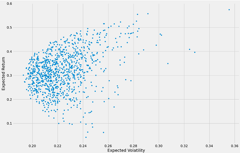

Portfolio Efficient Frontier: Expected Return (y) vs Volatility (x)

Calculating and plotting the minimum volatility portfolio (red star marker) vs the efficient frontier

min_vol_port = portfolios.iloc[portfolios['Volatility'].idxmin()]
# idxmin() gives us the minimum value in the column specified.                               
min_vol_port

Return        0.301451
Volatility    0.192731
Name: 670, dtype: float64

plt.subplots(figsize=[10,10])
plt.scatter(portfolios['Volatility'], portfolios['Return'],marker='o', s=20, alpha=0.7)
plt.scatter(min_vol_port[1], min_vol_port[0], color='r', marker='*', s=500);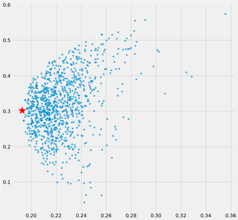

Portfolio Min Volatility vs Efficient Frontier: Volatility (x) vs Return (y).

Finding and plotting the minimum volatility portfolio (red star marker) vs the optimal risky portfolio (green star marker) overlaid by the efficient frontier

# Finding the optimal portfolio
rf = 0.01 # risk factor
optimal_risky_port = portfolios.iloc[((portfolios['Return']-rf)/portfolios['Volatility']).idxmax()]
optimal_risky_port

Return        0.458918
Volatility    0.224676
Name: 42, dtype: float64

# Plotting the optimal portfolio
plt.subplots(figsize=(10, 10))
plt.scatter(portfolios['Volatility'], portfolios['Return'],marker='o', s=20, alpha=0.7)
plt.scatter(min_vol_port[1], min_vol_port[0], color='r', marker='*', s=500)
plt.scatter(optimal_risky_port[1], optimal_risky_port[0], color='g', marker='*', s=500);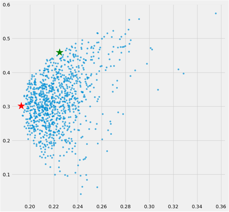

The minimum volatility portfolio (red star marker) vs the optimal risky portfolio (green star marker) overlaid by the efficient frontier: Volatility (x) vs Return (y).

Conclusions

We have calculated the risk adjusted return using the PyPortfolioOpt efficient frontier.
We have optimized a diversified 1Y portfolio of the following 5 US stocks: XOM, LMT, AAPL , LYTS, and VRTX.
Our optimal risky portfolio yields

Return        0.458918
Volatility    0.224676

Despite the wide use of Sharpe Ratios to compute risk adjusted returns, it is not without its disadvantages. Thus, if the expected returns do not follow a normal distribution or if the portfolios possess non-linear risks, the present PO approach may not deliver results.
The Road Ahead: Constrained Portfolio Optimization (CPO). Besides the objectives of maximizing return and minimizing risk, CPO is constrained by the investor’s preference for certain asset classes or assets.

Explore More

References

Contacts

Disclaimer

The following disclaimer clarifies that the information provided in this article is for educational use only and should not be considered financial or investment advice.
The information provided does not take into account your individual financial situation, objectives, or risk tolerance.
Any investment decisions or actions you undertake are solely your responsibility.
You should independently evaluate the suitability of any investment based on your financial objectives, risk tolerance, and investment timeframe.
It is recommended to seek advice from a certified financial professional who can provide personalized guidance tailored to your specific needs.
The tools, data, content, and information offered are impersonal and not customized to meet the investment needs of any individual. As such, the tools, data, content, and information are provided solely for informational and educational purposes only.