Algorithmic trading simplified: Value at Risk and Portfolio Optimization

In the last post, we saw how actual algorithms are developed and tested. In this post, we will figure out the level of exposure so that can always protect our investments from significant downturns. And find the best performing portfolio given several assets.

Why quantify the risk?

To invest or trade with confidence. Knowing Value at Risk (VaR) helps us to gauge the potential loss of equity, both in scale and frequency. Not managing this volatility can lead to significant (and avoidable) losses.

Why Optimize Portfolio?

We are all risk-averse and we want to maximize our profits. Diversification can potentially achieve both of these goals. We can select assets with the best returns that are less correlated with each other. Portfolio return and risk however depend upon final mix or weight allocation to each asset. Not getting allocation right will lead to lower returns/higher risks. We will use mean-variance optimization to find desired weights to construct the best performing portfolio(modern portfolio theory by Markowitz).

Short explanation/definition of key terms

Value at Risk (VaR): Maximum dollar amount (or percentage) expected to be lost over a given time horizon, at a pre-defined confidence/probability level.

Portfolio optimization and efficient frontier: Finding best weights for selected assets such that the expected return is highest for a given risk or vice versa. An efficient frontier is simply a collection of all such dominant/optimized portfolios for all possible risk level.

Sharpe ratio: Sharpe ratio is the measure of risk-adjusted return of a portfolio. Degree of excess return beyond risk-free asset for taking extra risk.

Capital Market Line (CML): Theoretical concept that gives optimal combinations of a risk-free asset and the market portfolio (portfolio of risky assets).

Convex optimization: Solving a mean-variance problem as convex functions, here with the help of Solvers.

Part 1: Value at Risk (VaR)

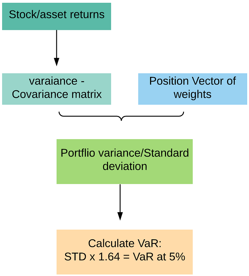
VaR represents portfolio variance at one extreme (of the distribution). Portfolio risk is calculated as portfolio variance (equivalently standard deviation). Portfolio variance plays a major role in determining the risk characteristic of asset as a whole. Portfolio variance depends upon variance of each asset within the portfolio as well their covariance. Thus when assets are uncorrelated (do not tend to move together) portfolio risks are lower compared to portfolio of assets are highly positively correlated.

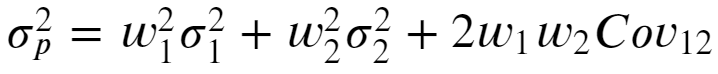
For a 2 asset portfolio, portfolio variance is given by following equation where w1, w2 are weights, sigma1, sigma2 are standard deviation of each asset and Cov12 denotes covariance between them.

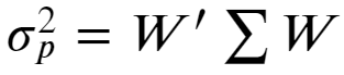
For multiple asset portfolio, position vector and covariance matrix make it much easier to express portfolio variance rather than writing a long summation.

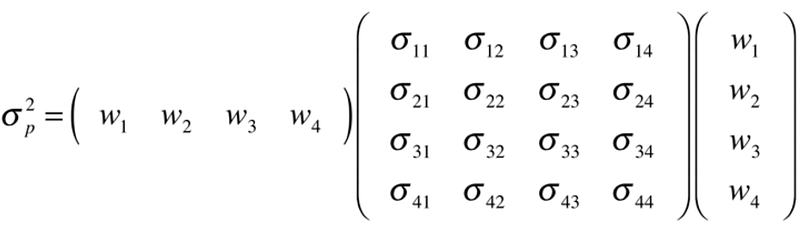
Following is an expanded view of the matrix operation.

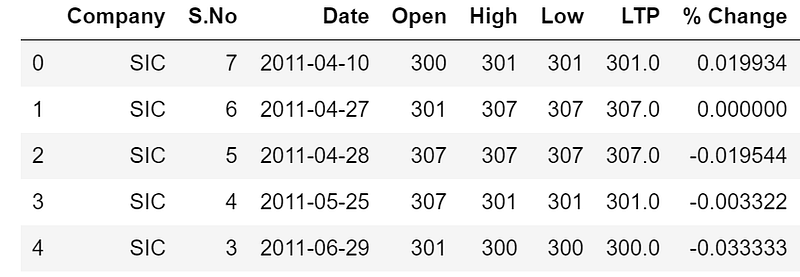
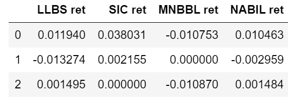
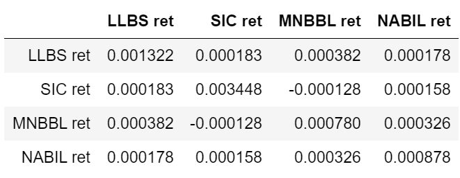
With python (Pandas/Numpy or other tools) it is straight forward to calculate the covariance matrix for the whole asset given the series of returns. Matrix multiplication is then used to get portfolio variance. For illustration, I have taken stocks from the Nepal Stock Exchange (NEPSE). 4 highly traded stocks from different sectors were selected. The process involves loading data, calculating return for each stock, computing covariance, and finally calculating portfolio variance as given below.

Data, returns and covariance can be seen in following tables.

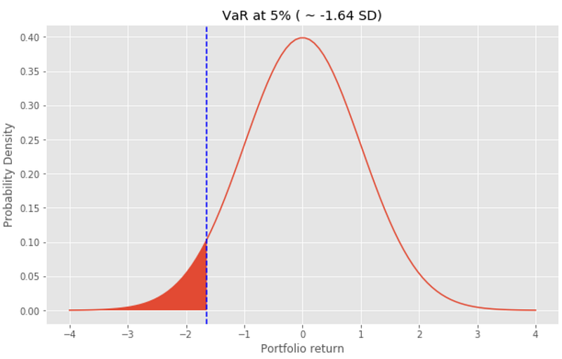
While standard deviation tells how much asset can fluctuate every day on average, VaR represents how much asset can fall a single day during a highly volatile period. VaR is expressed as a potential loss of asset (e.g. 4% of the total asset) with a certain probability (e.g. 2% chance or 98% confidence) within a certain time frame (e.g. daily/weekly). Being aware of VaR allows us to keep the right-sized asset or the right mix of assets such that we can avoid unexpected and huge losses. The image below shows that return could be as worse as or worse than -1.64 standard deviation 1 out of 20 trading days (5% probability).

It is obvious that we would want a portfolio and with minimum VaR as possible for any given return. Next, we will find such a portfolio with an optimal combination of weights that has a minimum variance for a specific return. Alternatively, portfolio optimization will help us to maximize our return for any selected risk level.

Example: For some random positions(weights) in 4 stocks [0.08, 0.2, 0.58, 0.14] calculated portfolio variance is 0.005, and standard deviation is 0.022 or 2.2% daily std. Assuming a normal distribution of returns, the worst 5% outcomes lie -1.64 SD away from the center. That is returns can be worse than -0.0367 or -3.67% (-1.645*0.022) in 1/20 trading days (5% chance). If we have $100000 invested, our Var at 5% probability is $3670. In other words, we tend to lose $3670 (or more) once in every 20 trading days.

Part 2. Portfolio Optimization

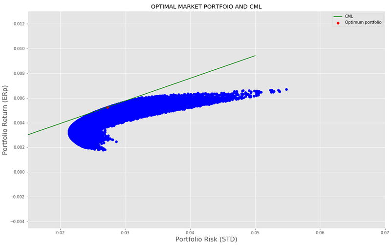
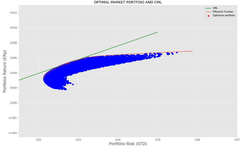
We will gradually discover the portfolio we want in few steps. We shall start with completely random allocation (i.e. use random weights). Some of these random weight portfolios have better risk-return trade-off, hence are dominant portfolios. Those lying most upper/outer in the risk-return plot make the efficient frontier. Next, we shall find the Market portfolio by comparing the Sharpe ratio for each random portfolio. Needless to say, the Market portfolio lies on the efficient frontier and has the highest/maximum Sharpe ratio. The line tangent to this point and passing through risk-free asset is the Capital Market Line. The slope and intercept to this line are Sharpe ratio and risk-free rate respectively. Ideally, all investors select their portfolio somewhere on this line depending upon their risk/return preferences.

A. Random allocation of weights: We will visualize the effect of random allocation weights. 1000s of portfolios are taken with random weights, respective mean and variance are calculated (and scattered for visualization). Some combination weight has better risk-return characteristics and therefore are dominating/desirable portfolios.

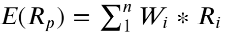
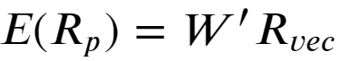
Portfolio return:

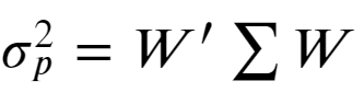
Portfolio risk:

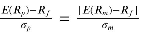
B. Market portfolio: Among all possible combinations of dominating portfolios in the efficient frontier, one which gives the highest return for taking additional risk beyond a risk-free rate is designated as a Market portfolio. we can calculate the Sharpe ratio for all portfolios given a risk-free rate and the winning portfolio with the highest Sharpe ratio is the Market Portfolio. All the rational investors gravitate towards to this best performing portfolio. This model of combining risk-free assets with the Market portfolio is known as the Capital asset pricing model (CAPM). All portfolios in CML is optimally compensated for risk above the risk-free rate. Mathematically CAPM is expressed as:

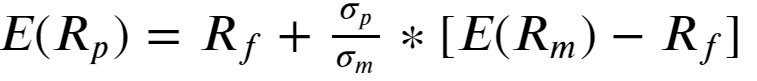
Rearranging, we have Sharpe ratio for combined portfolio :

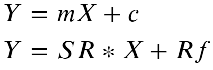
Using Rm and Sigma_m calculated from stock return and covariance Sharpe ratio for each random portfolio is calculated, one with the highest Sharpe ratio is the market/optimal portfolio. C. Capital Market Line (CML): Capital Market line represents all combinations of the risk-free asset and the optimal market portfolio. It’s easy to see that the slope of this line is the Sharpe ratio itself and the intercept is a risk-free rate. Given this information, CML can be readily drawn as seen below.

Code for constructing random portfolios, finding a market portfolio, and drawing CML line.

Part 3. Solvers

Random initialization of weights can work for a portfolio with few assets but when assets grow large, the cost of computing and time it takes can be forbidding. However, solving for the best portfolio is an optimization problem with constraints. We can use Solvers from python either for getting single best return (or risk) or get the entire efficient frontier. These are solved as convex problems and the global optimum is always reached.

The optimization objective is expressed as:

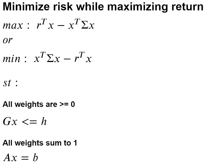
Here weights are represented by x and we are solving for optimal x. Objectives and constraints are written in matrix form. As a rule objective function is stated as a minimization problem. All the inequalities are similarly stated as lesser than some value.

Inputs for Solvers:

The algorithm solves for ‘x’ with the help of inputs

P or quadratic part (here it’s sigma or variance-covariance matrix, cov)

q or linear part of the objective function (here represented by a vector of returns r or ER_stocks, above)

G and h make the lower bound for weights i.e 0. We can input G as an identity matrix of size n x n (n: number of weights/stocks). Stated as matmul(G, x) < h, hence h is a vector of 0s of size n. while weights are non-negative, while solving they are stated as: -weights < 0.

A and b make the equality part of the constraint. For our purpose the sum of all weights must equal 1. Hence A is a vector of 1s of size n. matmul(A, r_transpose) = 1, or b is simply 1.

We can get the frontier and plot along with random portfolios:

Code to solve using Solvers.

Limitations and Conclusion

The biggest limitations of this model are the assumption of a normal distribution of returns and the validity of covariance. Actual returns are rarely normal and in fact, highly negative and positive returns are much more common giving rise to so-called fat-tailed distribution. As such the model underestimates the risks. Portfolio variance/risk is very sensitive to variance and covariance pairs i.e. the covariance matrix. Covariance rarely remains the same for a long time, hence finding a robust/valid covariance matrix is challenging.

Despite some limitations, risk modeling with VaR is a very helpful and probably most used indicator. Portfolio optimization leads to the most efficient use of our resources and any allocation decisions should be based upon these considerations. Solvers can be used to quickly find the efficient frontier or market portfolio has given return series for each stock.

You can read the earlier post here: