
Integration of Stochastic VaR Predictions, Quantstats Profit-Volatility Analysis & Backtesting of Disparity Index / Super Trend Trading Signals
Biotech R&D AZN Algo-Trading Use-Case Study: Beta Coefficient, VaR, Q-Q Plots, Monte Carlo Random Walk Simulations, Quantstats & Disparity Index (DI), Super Trend (ST) Backtesting vs SPY Benchmark

- “I’m an investor in a number of biotech companies, partly because of my incredible enthusiasm for the great innovations they will bring.”
- Bill Gates
- This post explores the application of algo-trading and fintech [3–6] to biotech, unraveling the unique trading/investment opportunities thanks to recent advances in biological science that could help the world overcome its most pressing challenges in health and sustainability [1,2].
- In its broadest definition, biotechnology is the use of advances in molecular biology for applications in human and animal health, agriculture, environment, and specialty biochemical manufacturing.
- Today our focus is on AstraZeneca PLC (NASDAQ:AZN) leading R&D in the biotech/biopharma industry. AZN, headquartered in London, UK, is one of the largest biopharmaceutical companies in the world.
- Zacks Review: AZN is a #3 (Hold) on the Zacks Rank, with a VGM Score of A. Additionally, the company could be a top pick for growth investors. AZN has a Growth Style Score of B, forecasting year-over-year earnings growth of 11.6% for the current fiscal year. AZN should be on investors’ short list.
Project Scope
- quantstats fin analysis: kurtosis, skewness, Beta, and Sharpe Ratio.
- Comparing normal and student probability Q-Q plots of daily returns.
- Monte Carlo simulation of random portfolios and VaR.
- Backtesting DI14/ST Trading Signals vs SPY Benchmark.
Let’s delve into the specifics of our financial analysis with a Python source code explanation on a line-by-line basis.
Basic Imports & Settings
- Importing/installing necessary Python libraries and setting default parameters
import numpy as np
import requests
import pandas as pd
import matplotlib.pyplot as plt
from math import floor
from termcolor import colored as cl
from scipy import stats
import quantstats as qs


import os
os.chdir('YOURPATH')    # Set working directory
os. getcwd()

plt.style.use('fivethirtyeight')
plt.rcParams['figure.figsize'] = (16,10)

import datetime as dt
import warnings
warnings.filterwarnings("ignore")
Fetching Stock Data
- Using twelvedata.com API to extract the AZN stock data [4,5]
def get_historical_data(symbol, start_date):
    api_key = 'YOUR API KEY'
    api_url = f'https://api.twelvedata.com/time_series?symbol={symbol}&interval=1day&outputsize=5000&apikey={api_key}'
    raw_df = requests.get(api_url).json()
    df = pd.DataFrame(raw_df['values']).iloc[::-1].set_index('datetime').astype(float)
    df = df[df.index >= start_date]
    df.index = pd.to_datetime(df.index)
    return df

googl = get_historical_data('AZN', '2022-01-01')
googl.tail()

           open  high  low   close  volume
datetime
2024-07-12 79.52 79.79 79.18 79.24 3051600.0
2024-07-15 79.15 79.15 78.04 78.12 2666900.0
2024-07-16 77.96 78.69 77.92 78.59 2668700.0
2024-07-17 78.50 79.83 78.50 79.76 3658900.0
2024-07-18 80.00 80.01 77.99 78.06 3231400.0

googl['close'].plot()
plt.title("AZN Close Price", weight="bold");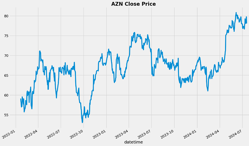
Daily Returns & STD
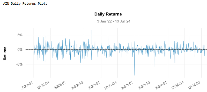
- Calculating the AZN daily returns
fig = plt.figure()
fig.set_size_inches(16,10)
googl['close'].pct_change().plot()
plt.title("AZN Daily Returns", weight="bold");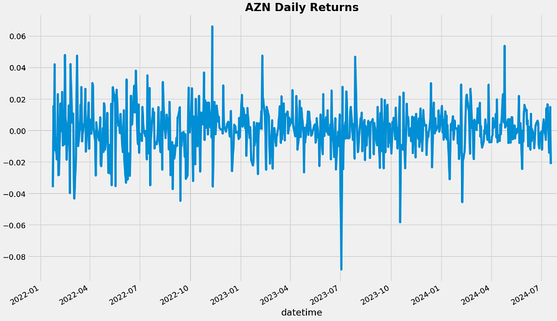
- Plotting the histogram of AZN daily returns and calculating STD [6]
googl['close'].pct_change().hist(bins=50, density=True, histtype="stepfilled", alpha=0.5)
plt.title("Histogram of AZN Daily Returns", weight="bold")
googl['close'].pct_change().std()

0.015141837172713706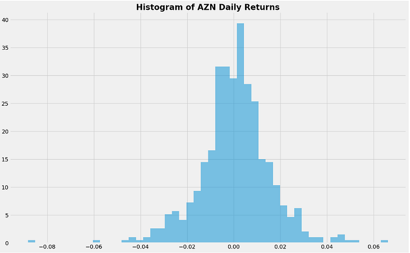
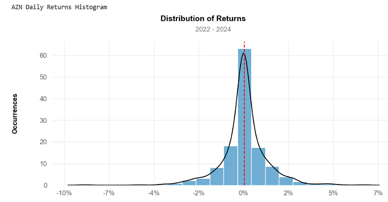
- Calculating the PDF parameters [6] and 5% quantile of AZN daily returns
returns = googl["close"].pct_change().dropna()
mean = returns.mean()
sigma = returns.std()
tdf, tmean, tsigma = scipy.stats.t.fit(returns)

returns.quantile(0.05)

-0.024858792323295287

support = numpy.linspace(returns.min(), returns.max(), 100)
returns.hist(bins=40, density=True, histtype="stepfilled", alpha=0.5);
plt.plot(support, scipy.stats.t.pdf(support, loc=tmean, scale=tsigma, df=tdf), "r-")
plt.title("Daily change in AZN (%)", weight="bold");

print (mean,sigma)

0.0005600276512388191 0.015141837172713706

scipy.stats.norm.ppf(0.05, mean, sigma)

-0.02434607814100796
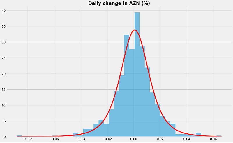
- Here, we calculate empirical quantiles from a histogram of daily returns. The 0.05 empirical quantile of daily returns is at -0.0248. That means that with 95% confidence, our worst daily loss will not exceed 2.5%. If we have a $1k investment, our one-day 5% VaR is 0.025 * $1k = $25.
- We calculate analytic quantiles by curve fitting to historical data (cf. red curve above). Here, we use Student’s t distribution (read below that it represents daily returns relatively well).
Normal/Student Probability Q-Q Plots
- Comparing normal and Student probability Q-Q plots [6]
Q = googl['close'].pct_change().dropna()
scipy.stats.probplot(Q, dist=scipy.stats.norm, plot=plt.figure().add_subplot(111))
plt.title("Normal probability plot of AZN Daily Returns", weight="bold");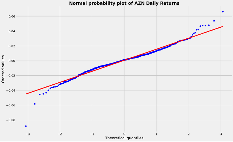
tdf, tmean, tsigma = scipy.stats.t.fit(Q)
scipy.stats.probplot(Q, dist=scipy.stats.t, sparams=(tdf, tmean, tsigma), plot=plt.figure().add_subplot(111))
plt.title("Student Probability Plot of AZN Daily Returns", weight="bold");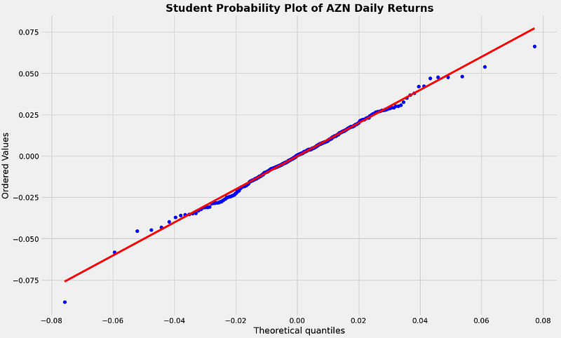
- Q-Q plots are particularly useful for assessing the normality of a dataset. If the data points in the plot closely follow a straight line, it indicates that the dataset is approximately normally distributed. Deviations from the line suggest departures from normality, which may require further investigation or non-parametric statistical techniques.
- We can see that the Student t-distribution (bottom plot) is closer to the straight line than the normal distribution (top plot).
- This means that the AZN daily returns are better represented by a Student-t distribution than by a normal distribution.
- Student t-distributions are known to have a greater chance for extreme values than normal distributions, and as a result have fatter tails.
Monte Carlo Simulation
- Performing the 1Y Monte Carlo simulation [6] of the AZN Close price
#We start by defining some parameters of the geometric Brownian motion
days = 300   # time horizon
dt = 1/float(days)
sigma = 0.015141837172713706 # volatility
mu = 0.0005600276512388191  # drift (average growth rate)
startprice=78.35

# Random Walk Simulation (RWS)

def random_walk(startprice):
    price = numpy.zeros(days)
    shock = numpy.zeros(days)
    price[0] = startprice
    for i in range(1, days):
        shock[i] = numpy.random.normal(loc=mu * dt, scale=sigma * numpy.sqrt(dt))
        price[i] = max(0, price[i-1] + shock[i] * price[i-1])
    return price

for run in range(10000):
    plt.plot(random_walk(startprice))
plt.xlabel("Days")
plt.ylabel("Price USD");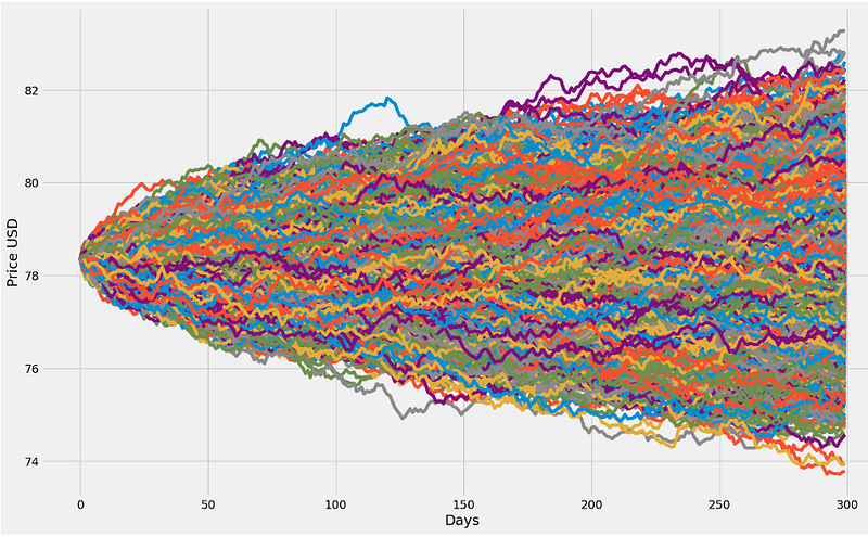
- Final price is spread out between $74 (our portfolio has lost value) to almost $83. We expect a profit because of the fact that the drift in our random walk (parameter mu) is positive.
AZN VaR Prediction
- Simulating the mean final price, VaR(0.99) and q(0.99) after 300 days [6]
runs = 10000
simulations = numpy.zeros(runs)
for run in range(runs):
    simulations[run] = random_walk(startprice)[days-1]
q = numpy.percentile(simulations, 1)
plt.hist(simulations, density=True, bins=30, histtype="stepfilled", alpha=0.5)
plt.figtext(0.6, 0.8, "Start price: $78.35")
plt.figtext(0.6, 0.7, "Mean final price: ${:.3}".format(simulations.mean()))
plt.figtext(0.6, 0.6, "VaR(0.99): ${:.3}".format(10 - q))
plt.figtext(0.15, 0.6, "q(0.99): ${:.3}".format(q))
plt.axvline(x=q, linewidth=4, color="r")
plt.title("Final price distribution after {} days".format(days), weight="bold");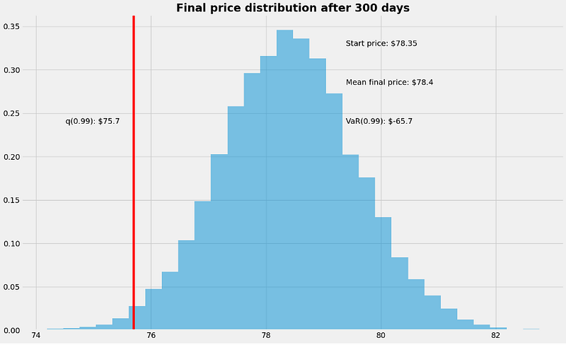
- We have looked at the 1% empirical quantile of the final price distribution to estimate VaR.
- VaR(0.99) is defined as the maximum dollar amount expected to be lost over a given time horizon, at a pre-defined confidence level. For example, if the 99% one-day VAR is $1k, there is 99% confidence that over the next month the portfolio will not lose more than $1k.
- A negative VaR would imply the stock has a high probability of making a profit, for example a one-day 1% VaR of negative $65.7 implies the portfolio has a 99% chance of making more than $65.7 over the next day.
Quantstats Financial Analysis
- Using quantstats to calculate the AZN cumulative returns, kurtosis/skewness of daily returns, STD, Sharpe Ratio, alpha and beta vs S&P 500 [3].
- Downloading and plotting the AZN daily returns
aapl = qs.utils.download_returns('AZN')
aapl = aapl.loc['2022-01-01':'2024-07-20']

# Converting timezone
aapl.index = aapl.index.tz_localize(None)

print('\nAZN Daily Returns Plot:\n')
qs.plots.daily_returns(aapl,benchmark='SPY')
- Plotting the AZN cumulative returns
print('\nAZN Cumulative Returns Plot\n')
qs.plots.returns(aapl)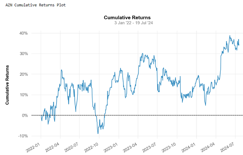
- We can see that that the AZN cumulative returns is ~35% over a given time horizon.
- Plotting the histogram of daily returns
- Calculating kurtosis, skewness, STD, and Sharpe Ratio
print("AZN's kurtosis: ", qs.stats.kurtosis(aapl).round(2))

AZN's kurtosis:  3.16

print("AZN's skewness: ", qs.stats.skew(aapl).round(2))

AZN's skewness:  -0.23

print("AZN's Standard Deviation: ", aapl.std())

AZN's Standard Deviation:  0.01507339590886966


print("Sharpe Ratio for AZN: ", qs.stats.sharpe(aapl).round(2))

Sharpe Ratio for AZN: 0.61- A Sharpe ratio of less than one is considered bad. The risk AZN encounters isn’t being offset well enough by its return. The higher the Sharpe ratio, the better.
- A standard normal distribution has kurtosis of 3 and is recognized as mesokurtic. An increased kurtosis (>3) can be visualized as a thin “bell” with a high peak.
- Skewness is a statistical measure of the asymmetry of a probability distribution. Skewness between -0.5 and 0.5 is symmetrical.
- There is strong evidence of a negative cross-sectional relationship between realized skewness and future stock returns — stocks with negative skewness are compensated with high future returns for higher volatility.
- Calculating alpha and beta vs SPY
sp500 = qs.utils.download_returns('SPY')
sp500 = sp500.loc['2022-01-01':'2024-07-20']
sp500.index = sp500.index.tz_localize(None)
sp500.tail()

Date
2024-07-15    0.002750
2024-07-16    0.005930
2024-07-17   -0.014021
2024-07-18   -0.007685
2024-07-19   -0.003185
Name: Close, dtype: float64

# Removing indexes
sp500_no_index = sp500.reset_index(drop = True)
aapl_no_index = aapl.reset_index(drop = True)

# Fitting linear relation among AZN's returns and Benchmark
X = sp500_no_index.values.reshape(-1,1)
y = aapl_no_index.values.reshape(-1,1)

linreg = LinearRegression().fit(X, y)

beta = linreg.coef_[0]
alpha = linreg.intercept_
print('\n')
print('AZN beta: ', beta.round(3))
print('\nAZN alpha: ', alpha.round(3))

AZN beta:  [0.498]

AZN alpha:  [0.]

y_pred = linreg.predict(X)

# Plot outputs
plt.scatter(X, y, color="blue",label='Observed')
plt.plot(X, y_pred, color="red", linewidth=3,label='Linear Regression')
plt.xlabel('SPY Daily Returns')
plt.ylabel('AZN Daily Returns')
plt.legend()
plt.grid(color='black')
plt.show()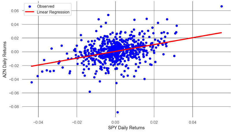
- A beta of less than 1 indicates that a stock’s price is less volatile than the overall market.
- A stock with an alpha of zero performs in line with the market.
Backtesting Disparity Index
- Let’s look at the Disparity Index (DI) trading strategy [4].
- DI is a momentum indicator that measures the relative position of an asset’s most recent closing price to a selected moving average and reports the value as a percentage.
- Calculating DI with lookback=14 (DI14)
ef get_di(data, lookback):
    ma = data.rolling(lookback).mean()
    di = ((data - ma) / ma) * 100
    return di

googl['di_14'] = get_di(googl['close'], 14)
googl = googl.dropna()
googl.tail()

           open   high low  close  volume    di_14
datetime
2024-07-12 79.52 79.79 79.18 79.24 3051600.0 1.573931
2024-07-15 79.15 79.15 78.04 78.12 2666900.0 0.252997
2024-07-16 77.96 78.69 77.92 78.59 2668700.0 0.963515
2024-07-17 78.50 79.83 78.50 79.76 3658900.0 2.402700
2024-07-18 80.00 80.01 77.99 78.06 3231400.0 0.231125- Here, di_14>0 shows that the price is rising, suggesting that the asset is gaining upward momentum. Conversely, di_14<0 can be interpreted as a sign that selling pressure is increasing, forcing the price to drop. A value di_14=0 means that the asset’s current price is exactly consistent with its moving average.
- Reading the input stocks data
googl = get_historical_data('AZN', '2022-01-01')
googl.tail()

open high low close volume
datetime
2024-07-15 79.15 79.15 78.04 78.12 2666900.0
2024-07-16 77.96 78.69 77.92 78.59 2668700.0
2024-07-17 78.50 79.83 78.50 79.76 3658900.0
2024-07-18 80.00 80.01 77.99 78.06 3232900.0
2024-07-19 78.34 78.76 78.16 78.71 2929800.0- Implementing the DI14 trading strategy and plotting the corresponding trading signals [4]
def implement_di_strategy(prices, di):
    buy_price = []
    sell_price = []
    di_signal = []
    signal = 0

    for i in range(len(prices)):
        if di[i-4] < 0 and di[i-3] < 0 and di[i-2] < 0 and di[i-1] < 0 and di[i] > 0:
            if signal != 1:
                buy_price.append(prices[i])
                sell_price.append(np.nan)
                signal = 1
                di_signal.append(signal)
            else:
                buy_price.append(np.nan)
                sell_price.append(np.nan)
                di_signal.append(0)
        elif di[i-4] > 0 and di[i-3] > 0 and di[i-2] > 0 and di[i-1] > 0 and di[i] < 0:
            if signal != -1:
                buy_price.append(np.nan)
                sell_price.append(prices[i])
                signal = -1
                di_signal.append(signal)
            else:
                buy_price.append(np.nan)
                sell_price.append(np.nan)
                di_signal.append(0)
        else:
            buy_price.append(np.nan)
            sell_price.append(np.nan)
            di_signal.append(0)

    return buy_price, sell_price, di_signal

buy_price, sell_price, di_signal = implement_di_strategy(googl['close'], googl['di_14'])

ax1 = plt.subplot2grid((11,1), (0,0), rowspan = 5, colspan = 1)
ax2 = plt.subplot2grid((11,1), (6,0), rowspan = 5, colspan = 1)
ax1.plot(googl['close'], linewidth = 2, color = '#1976d2')
ax1.plot(googl.index, buy_price, marker = '^', markersize = 12, linewidth = 0, label = 'BUY SIGNAL', color = 'green')
ax1.plot(googl.index, sell_price, marker = 'v', markersize = 12, linewidth = 0, label = 'SELL SIGNAL', color = 'r')
ax1.legend()
ax1.set_title('AZN CLOSING PRICES')
for i in range(len(googl)):
    if googl.iloc[i, 5] >= 0:
        ax2.bar(googl.iloc[i].name, googl.iloc[i, 5], color = '#26a69a')
    else:
        ax2.bar(googl.iloc[i].name, googl.iloc[i, 5], color = '#ef5350')
ax2.set_title('AZN DISPARITY INDEX 14')
plt.show()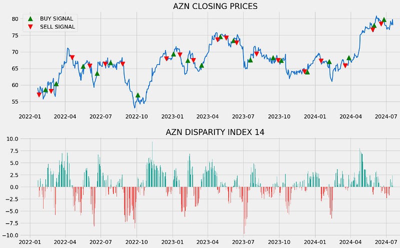
- Calculating the AZN stock position based on the above trading signals
position = []
for i in range(len(di_signal)):
    if di_signal[i] > 1:
        position.append(0)
    else:
        position.append(1)

for i in range(len(googl['close'])):
    if di_signal[i] == 1:
        position[i] = 1
    elif di_signal[i] == -1:
        position[i] = 0
    else:
        position[i] = position[i-1]

close_price = googl['close']
di = googl['di_14']
di_signal = pd.DataFrame(di_signal).rename(columns = {0:'di_signal'}).set_index(googl.index)
position = pd.DataFrame(position).rename(columns = {0:'di_position'}).set_index(googl.index)

frames = [close_price, di, di_signal, position]
strategy = pd.concat(frames, join = 'inner', axis = 1)

strategy.tail()

          close   di_14 di_signal di_position
datetime
2024-07-12 79.24 1.573931 0 1
2024-07-15 78.12 0.252997 0 1
2024-07-16 78.59 0.963515 0 1
2024-07-17 79.76 2.402700 0 1
2024-07-18 78.06 0.231125 0 1
2024-07-19 78.71 0.999047 0 1- Backtesting the DI14 trading strategy
googl_ret = pd.DataFrame(np.diff(googl['close'])).rename(columns = {0:'returns'})
di_strategy_ret = []

for i in range(len(googl_ret)):
    returns = googl_ret['returns'][i]*strategy['di_position'][i]
    di_strategy_ret.append(returns)

di_strategy_ret_df = pd.DataFrame(di_strategy_ret).rename(columns = {0:'di_returns'})
investment_value = 10000
number_of_stocks = floor(investment_value/googl['close'][0])
di_investment_ret = []

for i in range(len(di_strategy_ret_df['di_returns'])):
    returns = number_of_stocks*di_strategy_ret_df['di_returns'][i]
    di_investment_ret.append(returns)

di_investment_ret_df = pd.DataFrame(di_investment_ret).rename(columns = {0:'investment_returns'})
total_investment_ret = round(sum(di_investment_ret_df['investment_returns']), 2)
profit_percentage = floor((total_investment_ret/investment_value)*100)
print(cl('Profit gained from the DI14 strategy by investing $10k in AZN : {}'.format(total_investment_ret), attrs = ['bold']))
print(cl('Profit percentage of the AZN strategy : {}%'.format(profit_percentage), attrs = ['bold']))

Profit gained from the DI14 strategy by investing $10k in AZN : 5480.67
Profit percentage of the DI14 strategy : 54%- Benchmarking the DI14 trading strategy vs SPY
def get_benchmark(start_date, investment_value):
    spy = get_historical_data('SPY', start_date)['close']
    benchmark = pd.DataFrame(np.diff(spy)).rename(columns = {0:'benchmark_returns'})

    investment_value = investment_value
    number_of_stocks = floor(investment_value/spy[-1])
    benchmark_investment_ret = []

    for i in range(len(benchmark['benchmark_returns'])):
        returns = number_of_stocks*benchmark['benchmark_returns'][i]
        benchmark_investment_ret.append(returns)

    benchmark_investment_ret_df = pd.DataFrame(benchmark_investment_ret).rename(columns = {0:'investment_returns'})
    return benchmark_investment_ret_df

benchmark = get_benchmark('2022-01-01', 10000)
investment_value = 10000
total_benchmark_investment_ret = round(sum(benchmark['investment_returns']), 2)
benchmark_profit_percentage = floor((total_benchmark_investment_ret/investment_value)*100)
print(cl('Benchmark profit by investing $10k : {}'.format(total_benchmark_investment_ret), attrs = ['bold']))
print(cl('Benchmark Profit percentage : {}%'.format(benchmark_profit_percentage), attrs = ['bold']))
print(cl('DI14 Strategy profit is {}% higher than the Benchmark Profit'.format(profit_percentage - benchmark_profit_percentage), attrs = ['bold']))

Benchmark profit by investing $10k : 1283.04
Benchmark Profit percentage : 12%
DI14 Strategy profit is 42% higher than the Benchmark Profit- Comparing daily/cumulative returns of the DI14 vs Buy-Hold strategies
rets = googl['close'].pct_change().dropna()
strat_rets = strategy.di_position[1:]*rets
plt.figure(figsize=(12,6))
plt.title('Daily Returns')
rets.plot(color = 'blue', alpha = 0.3, linewidth = 7,label = 'BUY-HOLD')
strat_rets.plot(color = 'r', linewidth = 1,label = 'DI14 STRATEGY')
plt.legend(loc = 'lower left')
plt.show()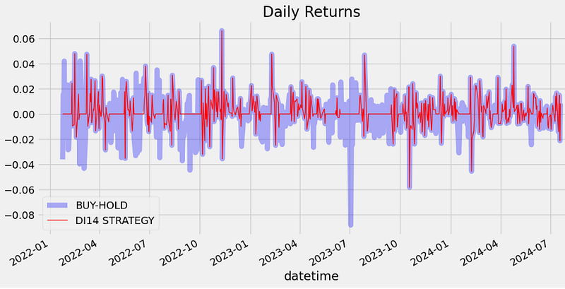
rets_cum = (1 + rets).cumprod() - 1
strat_cum = (1 + strat_rets).cumprod() - 1
plt.figure(figsize=(12,6))
plt.title('Cumulative Returns')
rets_cum.plot(color = 'blue', alpha = 0.3, linewidth = 7,label = 'BUY-HOLD')
strat_cum.plot(color = 'r', linewidth = 2,label = 'DI14 STRATEGY')
plt.legend(loc = 'upper left')
plt.show()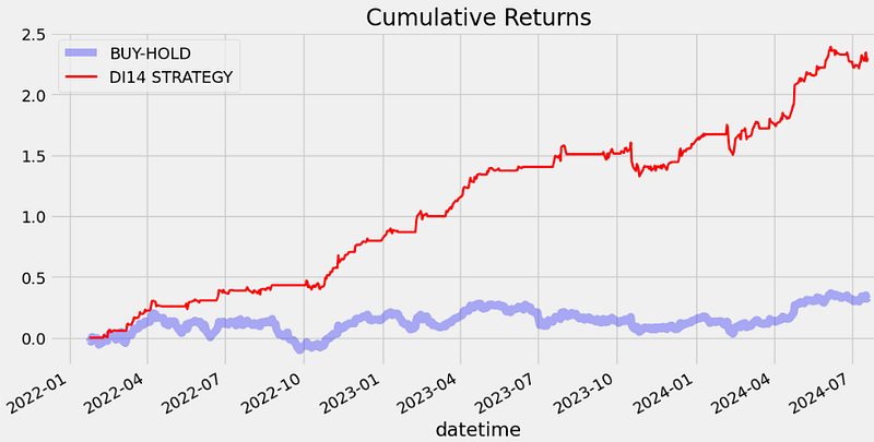
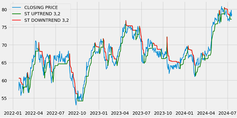
Backtesting Supertrend
- Supertrend (ST) is a trend-following indicator based on Average True Range (ATR). The calculation of its single line combines trend detection and volatility. It can be used to detect changes in trend direction and to position stops.
- Let’s evaluate the ST trading strategy [5].
- Reading the input data
aapl = get_historical_data('AZN', '2022-01-01')
aapl.tail()

           open  high  low   close  volume
datetime
2024-07-15 79.15 79.15 78.04 78.12 2666900.0
2024-07-16 77.96 78.69 77.92 78.59 2668700.0
2024-07-17 78.50 79.83 78.50 79.76 3658900.0
2024-07-18 80.00 80.01 77.99 78.06 3232900.0
2024-07-19 78.34 78.76 78.16 78.71 2929800.0- Calculating the ST indicator with the optimized values lookback=3 and multiplier=2 that maximize the expected return
def get_supertrend(high, low, close, lookback, multiplier):

    # ATR

    tr1 = pd.DataFrame(high - low)
    tr2 = pd.DataFrame(abs(high - close.shift(1)))
    tr3 = pd.DataFrame(abs(low - close.shift(1)))
    frames = [tr1, tr2, tr3]
    tr = pd.concat(frames, axis = 1, join = 'inner').max(axis = 1)
    atr = tr.ewm(lookback).mean()

    # H/L AVG AND BASIC UPPER & LOWER BAND

    hl_avg = (high + low) / 2
    upper_band = (hl_avg + multiplier * atr).dropna()
    lower_band = (hl_avg - multiplier * atr).dropna()

    # FINAL UPPER BAND

    final_bands = pd.DataFrame(columns = ['upper', 'lower'])
    final_bands.iloc[:,0] = [x for x in upper_band - upper_band]
    final_bands.iloc[:,1] = final_bands.iloc[:,0]

    for i in range(len(final_bands)):
        if i == 0:
            final_bands.iloc[i,0] = 0
        else:
            if (upper_band.iloc[i] < final_bands.iloc[i-1,0]) | (close.iloc[i-1] > final_bands.iloc[i-1,0]):
                final_bands.iloc[i,0] = upper_band.iloc[i]
            else:
                final_bands.iloc[i,0] = final_bands.iloc[i-1,0]

    # FINAL LOWER BAND

    for i in range(len(final_bands)):
        if i == 0:
            final_bands.iloc[i, 1] = 0
        else:
            if (lower_band.iloc[i] > final_bands.iloc[i-1,1]) | (close.iloc[i-1] < final_bands.iloc[i-1,1]):
                final_bands.iloc[i,1] = lower_band.iloc[i]
            else:
                final_bands.iloc[i,1] = final_bands.iloc[i-1,1]

    # SUPERTREND

    supertrend = pd.DataFrame(columns = [f'supertrend_{lookback}'])
    supertrend.iloc[:,0] = [x for x in final_bands['upper'] - final_bands['upper']]

    for i in range(len(supertrend)):
        if i == 0:
            supertrend.iloc[i, 0] = 0
        elif supertrend.iloc[i-1, 0] == final_bands.iloc[i-1, 0] and close.iloc[i] < final_bands.iloc[i, 0]:
            supertrend.iloc[i, 0] = final_bands.iloc[i, 0]
        elif supertrend.iloc[i-1, 0] == final_bands.iloc[i-1, 0] and close.iloc[i] > final_bands.iloc[i, 0]:
            supertrend.iloc[i, 0] = final_bands.iloc[i, 1]
        elif supertrend.iloc[i-1, 0] == final_bands.iloc[i-1, 1] and close.iloc[i] > final_bands.iloc[i, 1]:
            supertrend.iloc[i, 0] = final_bands.iloc[i, 1]
        elif supertrend.iloc[i-1, 0] == final_bands.iloc[i-1, 1] and close.iloc[i] < final_bands.iloc[i, 1]:
            supertrend.iloc[i, 0] = final_bands.iloc[i, 0]

    supertrend = supertrend.set_index(upper_band.index)
    supertrend = supertrend.dropna()[1:]

    # ST UPTREND/DOWNTREND

    upt = []
    dt = []
    close = close.iloc[len(close) - len(supertrend):]

    for i in range(len(supertrend)):
        if close.iloc[i] > supertrend.iloc[i, 0]:
            upt.append(supertrend.iloc[i, 0])
            dt.append(np.nan)
        elif close.iloc[i] < supertrend.iloc[i, 0]:
            upt.append(np.nan)
            dt.append(supertrend.iloc[i, 0])
        else:
            upt.append(np.nan)
            dt.append(np.nan)

    st, upt, dt = pd.Series(supertrend.iloc[:, 0]), pd.Series(upt), pd.Series(dt)
    upt.index, dt.index = supertrend.index, supertrend.index

    return st, upt, dt

aapl['st'], aapl['s_upt'], aapl['st_dt'] = get_supertrend(aapl['high'], aapl['low'], aapl['close'], 3, 2)
aapl = aapl[1:]
aapl.head()
plt.figure(figsize=(12,6))
plt.plot(aapl['close'], linewidth = 2, label = 'CLOSING PRICE')
plt.plot(aapl['st'], color = 'green', linewidth = 2, label = 'ST UPTREND 3,2')
plt.plot(aapl['st_dt'], color = 'r', linewidth = 2, label = 'ST DOWNTREND 3,2')
plt.legend(loc = 'upper left')
plt.show()
- Implementing the ST trading strategy by calculating ST trading signals, stock position and expected returns vs Buy-Hold strategy
def implement_st_strategy(prices, st):
buy_price = []
sell_price = []
st_signal = []
signal = 0
for i in range(len(st)):
if st.iloc[i-1] > prices.iloc[i-1] and st.iloc[i] < prices.iloc[i]:
if signal != 1:
buy_price.append(prices.iloc[i])
sell_price.append(np.nan)
signal = 1
st_signal.append(signal)
else:
buy_price.append(np.nan)
sell_price.append(np.nan)
st_signal.append(0)
elif st.iloc[i-1] < prices.iloc[i-1] and st.iloc[i] > prices.iloc[i]:
if signal != -1:
buy_price.append(np.nan)
sell_price.append(prices.iloc[i])
signal = -1
st_signal.append(signal)
else:
buy_price.append(np.nan)
sell_price.append(np.nan)
st_signal.append(0)
else:
buy_price.append(np.nan)
sell_price.append(np.nan)
st_signal.append(0)
return buy_price, sell_price, st_signal
buy_price, sell_price, st_signal = implement_st_strategy(aapl['close'], aapl['st'])
plt.figure(figsize=(12,6))
plt.plot(aapl['close'], linewidth = 2)
plt.plot(aapl['st'], color = 'green', linewidth = 2, label = 'ST UPTREND')
plt.plot(aapl['st_dt'], color = 'r', linewidth = 2, label = 'ST DOWNTREND')
plt.plot(aapl.index, buy_price, marker = '^', color = 'green', markersize = 12, linewidth = 0, label = 'BUY SIGNAL')
plt.plot(aapl.index, sell_price, marker = 'v', color = 'r', markersize = 12, linewidth = 0, label = 'SELL SIGNAL')
plt.title('ST TRADING SIGNALS')
plt.legend(loc = 'upper left')
plt.show()
position = []
for i in range(len(st_signal)):
if st_signal[i] > 1:
position.append(0)
else:
position.append(1)
for i in range(len(aapl['close'])):
if st_signal[i] == 1:
position[i] = 1
elif st_signal[i] == -1:
position[i] = 0
else:
position[i] = position[i-1]
close_price = aapl['close']
st = aapl['st']
st_signal = pd.DataFrame(st_signal).rename(columns = {0:'st_signal'}).set_index(aapl.index)
position = pd.DataFrame(position).rename(columns = {0:'st_position'}).set_index(aapl.index)
frames = [close_price, st, st_signal, position]
strategy = pd.concat(frames, join = 'inner', axis = 1)
strategy.head()
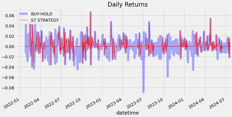
rets = aapl.close.pct_change().dropna()
strat_rets = strategy.st_position[1:]*rets
plt.figure(figsize=(12,6))
plt.title('Daily Returns')
rets.plot(color = 'blue', alpha = 0.3, linewidth = 7,label = 'BUY-HOLD')
strat_rets.plot(color = 'r', linewidth = 1,label = 'ST STRATEGY')
plt.legend(loc = 'upper left')
plt.show()
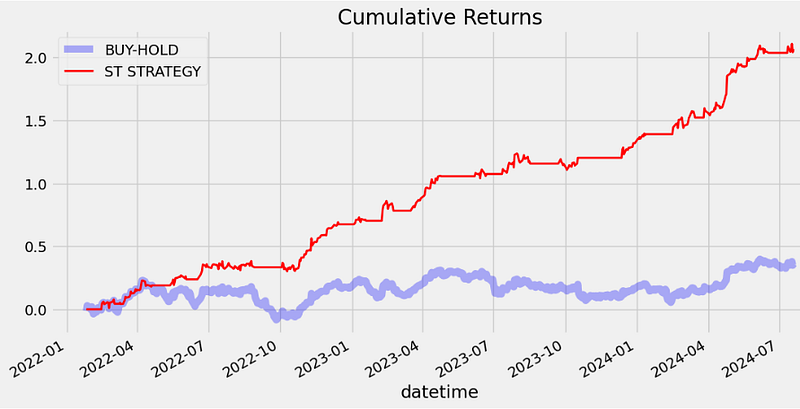
rets_cum = (1 + rets).cumprod() - 1
strat_cum = (1 + strat_rets).cumprod() - 1
plt.figure(figsize=(12,6))
plt.title('Cumulative Returns')
rets_cum.plot(color = 'blue', alpha = 0.3, linewidth = 7,label = 'BUY-HOLD')
strat_cum.plot(color = 'r', linewidth = 2,label = 'ST STRATEGY')
plt.legend(loc = 'upper left')
plt.show()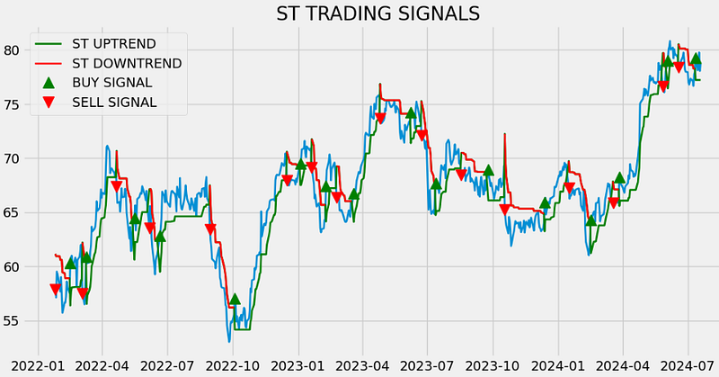
- Backtesting ST strategy
aapl_ret = pd.DataFrame(np.diff(aapl['close'])).rename(columns = {0:'returns'})
st_strategy_ret = []

for i in range(len(aapl_ret)):
    returns = aapl_ret['returns'][i]*strategy['st_position'][i]
    st_strategy_ret.append(returns)

st_strategy_ret_df = pd.DataFrame(st_strategy_ret).rename(columns = {0:'st_returns'})
investment_value = 10000
number_of_stocks = floor(investment_value/aapl['close'][0])
st_investment_ret = []

for i in range(len(st_strategy_ret_df['st_returns'])):
    returns = number_of_stocks*st_strategy_ret_df['st_returns'][i]
    st_investment_ret.append(returns)

st_investment_ret_df = pd.DataFrame(st_investment_ret).rename(columns = {0:'investment_returns'})
total_investment_ret = round(sum(st_investment_ret_df['investment_returns']), 2)
profit_percentage = floor((total_investment_ret/investment_value)*100)
print(cl('Profit gained from the ST strategy by investing $10k in AZN : {}'.format(total_investment_ret), attrs = ['bold']))
print(cl('Profit percentage of the ST strategy : {}%'.format(profit_percentage), attrs = ['bold']))

Profit gained from the ST strategy by investing $10k in AZN : 4262.16
Profit percentage of the ST strategy : 42%- Benchmarking ST strategy vs SPY
def get_benchmark(start_date, investment_value):
    spy = get_historical_data('SPY', start_date)['close']
    benchmark = pd.DataFrame(np.diff(spy)).rename(columns = {0:'benchmark_returns'})

    investment_value = investment_value
    number_of_stocks = floor(investment_value/spy[0])
    benchmark_investment_ret = []

    for i in range(len(benchmark['benchmark_returns'])):
        returns = number_of_stocks*benchmark['benchmark_returns'][i]
        benchmark_investment_ret.append(returns)

    benchmark_investment_ret_df = pd.DataFrame(benchmark_investment_ret).rename(columns = {0:'investment_returns'})
    return benchmark_investment_ret_df

benchmark = get_benchmark('2022-01-01', 10000)
investment_value = 10000
total_benchmark_investment_ret = round(sum(benchmark['investment_returns']), 2)
benchmark_profit_percentage = floor((total_benchmark_investment_ret/investment_value)*100)
print(cl('Benchmark profit by investing $10k : {}'.format(total_benchmark_investment_ret), attrs = ['bold']))
print(cl('Benchmark Profit percentage : {}%'.format(benchmark_profit_percentage), attrs = ['bold']))
print(cl('ST Strategy profit is {}% higher than the Benchmark Profit'.format(profit_percentage - benchmark_profit_percentage), attrs = ['bold']))

Benchmark profit by investing $10k : 1425.6
Benchmark Profit percentage : 14%
ST Strategy profit is 28% higher than the Benchmark Profit
Conclusions
- In this post, we have presented the detailed real-time AZN stock algo-trading analysis, including expected returns, kurtosis, skewness, STD, Sharpe Ratio, quantiles, Q-Q plots, beta and alpha vs SPY.
- We have estimated risk using a Monte Carlo simulation (MCS).
- We have calculated the value at risk (VaR) of AZN by running MCS that attempts to predict the worst likely loss for a portfolio given a confidence interval 99% over a time horizon of 300 days.
- We have implemented the DI14 and ST trading strategies for historical AZN Close prices 2022–2024.
- Our comparative analysis of backtesting and benchmarking tests has shown that ROI(DI14) (=54%) > ROI(ST) (=42%) > ROI(SPY) (=14%).
- The Road Ahead:
- Backtesting other trading strategies such as HFT, scalping, pairs trading, mean reversion, etc.
- Integrating ML/AI into algo-trading strategies, enhancing predictive capabilities.
- Exploring unconventional data streams, including sentiment analysis and geospatial information.
Acknowledgements
- Nikhil Adithyan @CodeX https://bit.ly/3yNuwCJ / GitHub
- Luís Fernando Torres
- Eric Marsden [email protected]
References
- Europe’s Bio Revolution: Biological innovations for complex problems
- The global landscape of biotech innovation: state of play
- Data Science for Financial Markets
- Algorithmic Trading with the Disparity Index in Python
- Algorithmic-Trading-with-Python/Overlap/SuperTrend.py
- Stock market trends and Value at Risk
Explore More
- Oracle Monte Carlo Stock Simulations
- Multiple-Criteria Technical Analysis of Blue Chips in Python
- Top 6 Reliability/Risk Engineering Learnings
- Data Visualization in Python — 1. Stock Technical Indicators
- Python Technical Analysis for Biotech — Get Buy Alerts on ABBV in 2023
- Biotech Genmab Hold Alert via Fibonacci Retracement Trading Simulations
- Applying a Risk-Aware Portfolio Rebalancing Strategy to ETF, Energy, Pharma, and Aerospace/Defense Stocks in 2023
- Quant Trading using Monte Carlo Predictions and 62 AI-Assisted Trading Technical Indicators (TTI)
Contacts
Disclaimer
- The following disclaimer clarifies that the information provided in this article is for educational use only and should not be considered financial or investment advice.
- The information provided does not take into account your individual financial situation, objectives, or risk tolerance.
- Any investment decisions or actions you undertake are solely your responsibility.
- You should independently evaluate the suitability of any investment based on your financial objectives, risk tolerance, and investment timeframe.
- It is recommended to seek advice from a certified financial professional who can provide personalized guidance tailored to your specific needs.
- The tools, data, content, and information offered are impersonal and not customized to meet the investment needs of any individual. As such, the tools, data, content, and information are provided solely for informational and educational purposes only.


