
Max Sharpe Portfolio of Top 10 Cryptos with Risk-Adjusted Weights

- This post is about crypto portfolio optimization using Modern Portfolio Theory (MPT) and its practical applications in the digital currency world.
- Specifically, we consider the max Sharpe Ratio portfolio (aka tangency portfolio) to calculate risk-adjusted returns on the efficient side of the mean-variance frontier, focusing on ten major cryptocurrencies from 2023–01–03 to 2024–05–19.
- Our objective is to create a diversified crypto portfolio and evaluate its performance. By adjusting and analyzing portfolio weights, we can make informed decisions that maximize the Return/Risk ratio.
Let’s delve into the details of the crypto portfolio optimization approach.
- Setting the working directory YOURPATH, importing libraries and reading the historical data of top 10 cryptos
import os
os.chdir('YOURPATH')    # Set working directory
os. getcwd()

mport yfinance as yf
import numpy as np
import pandas as pd
import os
import seaborn as sns

data = yf.download("BTC-USD ETH-USD USDT-USD USDC-USD BNB-USD BUSD-USD XRP-USD ADA-USD SOL-USD DOGE-USD", start="2023-01-03", end="2024-05-19")

data.tail()

Price Adj Close ... Volume
Ticker ADA-USD BNB-USD BTC-USD BUSD-USD DOGE-USD ETH-USD SOL-USD USDC-USD USDT-USD XRP-USD ... ADA-USD BNB-USD BTC-USD BUSD-USD DOGE-USD ETH-USD SOL-USD USDC-USD USDT-USD XRP-USD
Date
2024-05-15 0.452988 582.074341 66267.492188 1.000666 0.155526 3037.056641 158.186829 1.000128 1.000547 0.519004 ... 357450532 1895100260 39815167074 10177577 1767635344 14666902956 3585715674 8085028154 70663923975 1118098628
2024-05-16 0.459695 569.190247 65231.582031 1.000313 0.149637 2945.131104 159.116455 0.999971 1.000098 0.515698 ... 367462393 1911862000 31573077994 8840931 1374063837 13035465176 3498272951 6684369918 62000126842 1152212983
2024-05-17 0.482000 581.178345 67051.875000 1.000663 0.155563 3094.118652 169.530548 1.000018 1.000400 0.523804 ... 447612110 1557134929 28031279310 5423233 1112782871 14449438097 3371355809 6590780561 56249728895 1015239692
2024-05-18 0.482408 580.481140 66940.804688 1.000472 0.153077 3122.948975 172.539139 1.000082 1.000206 0.521390 ... 240076401 1358737176 16712277406 5423109 771261615 9407051320 2479657643 3748984171 39091871989 496850725
2024-05-19 0.467602 574.631653 66278.367188 1.000103 0.149107 3071.843018 170.091354 0.999953 0.999912 0.509661 ... 250323995 1298887094 19249094538 6368433 786457296 8747800800 2300080451 3531934053 38312293613 562911149
5 rows × 60 columns- Getting general info about the dataset
data.shape
(503, 60)

data.info()

<class 'pandas.core.frame.DataFrame'>
DatetimeIndex: 503 entries, 2023-01-03 to 2024-05-19
Data columns (total 60 columns):
 #   Column                 Non-Null Count  Dtype
---  ------                 --------------  -----
 0   (Adj Close, ADA-USD)   503 non-null    float64
 1   (Adj Close, BNB-USD)   503 non-null    float64
 2   (Adj Close, BTC-USD)   503 non-null    float64
 3   (Adj Close, BUSD-USD)  503 non-null    float64
 4   (Adj Close, DOGE-USD)  503 non-null    float64
 5   (Adj Close, ETH-USD)   503 non-null    float64
 6   (Adj Close, SOL-USD)   503 non-null    float64
 7   (Adj Close, USDC-USD)  503 non-null    float64
 8   (Adj Close, USDT-USD)  503 non-null    float64
 9   (Adj Close, XRP-USD)   503 non-null    float64
 10  (Close, ADA-USD)       503 non-null    float64
 11  (Close, BNB-USD)       503 non-null    float64
 12  (Close, BTC-USD)       503 non-null    float64
 13  (Close, BUSD-USD)      503 non-null    float64
 14  (Close, DOGE-USD)      503 non-null    float64
 15  (Close, ETH-USD)       503 non-null    float64
 16  (Close, SOL-USD)       503 non-null    float64
 17  (Close, USDC-USD)      503 non-null    float64
 18  (Close, USDT-USD)      503 non-null    float64
 19  (Close, XRP-USD)       503 non-null    float64
 20  (High, ADA-USD)        503 non-null    float64
 21  (High, BNB-USD)        503 non-null    float64
 22  (High, BTC-USD)        503 non-null    float64
 23  (High, BUSD-USD)       503 non-null    float64
 24  (High, DOGE-USD)       503 non-null    float64
 25  (High, ETH-USD)        503 non-null    float64
 26  (High, SOL-USD)        503 non-null    float64
 27  (High, USDC-USD)       503 non-null    float64
 28  (High, USDT-USD)       503 non-null    float64
 29  (High, XRP-USD)        503 non-null    float64
 30  (Low, ADA-USD)         503 non-null    float64
 31  (Low, BNB-USD)         503 non-null    float64
 32  (Low, BTC-USD)         503 non-null    float64
 33  (Low, BUSD-USD)        503 non-null    float64
 34  (Low, DOGE-USD)        503 non-null    float64
 35  (Low, ETH-USD)         503 non-null    float64
 36  (Low, SOL-USD)         503 non-null    float64
 37  (Low, USDC-USD)        503 non-null    float64
 38  (Low, USDT-USD)        503 non-null    float64
 39  (Low, XRP-USD)         503 non-null    float64
 40  (Open, ADA-USD)        503 non-null    float64
 41  (Open, BNB-USD)        503 non-null    float64
 42  (Open, BTC-USD)        503 non-null    float64
 43  (Open, BUSD-USD)       503 non-null    float64
 44  (Open, DOGE-USD)       503 non-null    float64
 45  (Open, ETH-USD)        503 non-null    float64
 46  (Open, SOL-USD)        503 non-null    float64
 47  (Open, USDC-USD)       503 non-null    float64
 48  (Open, USDT-USD)       503 non-null    float64
 49  (Open, XRP-USD)        503 non-null    float64
 50  (Volume, ADA-USD)      503 non-null    int64
 51  (Volume, BNB-USD)      503 non-null    int64
 52  (Volume, BTC-USD)      503 non-null    int64
 53  (Volume, BUSD-USD)     503 non-null    int64
 54  (Volume, DOGE-USD)     503 non-null    int64
 55  (Volume, ETH-USD)      503 non-null    int64
 56  (Volume, SOL-USD)      503 non-null    int64
 57  (Volume, USDC-USD)     503 non-null    int64
 58  (Volume, USDT-USD)     503 non-null    int64
 59  (Volume, XRP-USD)      503 non-null    int64
dtypes: float64(50), int64(10)
memory usage: 239.7 KB- Examining the summary statistics
data.describe().T

count mean std min 25% 50% 75% max
Price Ticker
Adj Close
ADA-USD 503.0 4.065172e-01 1.293618e-01 2.418730e-01 2.963965e-01 3.776930e-01 4.858075e-01 7.741900e-01
BNB-USD 503.0 3.208171e+02 1.150505e+02 2.052294e+02 2.402693e+02 3.023846e+02 3.249082e+02 6.328028e+02
BTC-USD 503.0 3.687814e+04 1.483931e+04 1.667986e+04 2.673656e+04 2.977180e+04 4.323705e+04 7.308350e+04
BUSD-USD 503.0 1.000826e+00 2.851725e-03 9.986540e-01 1.000009e+00 1.000249e+00 1.000627e+00 1.040575e+00
DOGE-USD 503.0 9.006512e-02 3.432984e-02 5.789700e-02 7.026600e-02 7.880600e-02 9.015200e-02 2.200640e-01
ETH-USD 503.0 2.133607e+03 6.274484e+02 1.214779e+03 1.670317e+03 1.873076e+03 2.337104e+03 4.066445e+03
SOL-USD 503.0 5.861475e+01 5.290410e+01 1.309227e+01 2.091821e+01 2.431775e+01 9.786334e+01 2.028741e+02
USDC-USD 503.0 9.999469e-01 1.334716e-03 9.715000e-01 9.999540e-01 1.000028e+00 1.000109e+00 1.000751e+00
USDT-USD 503.0 1.000231e+00 7.462615e-04 9.983820e-01 9.999810e-01 1.000159e+00 1.000396e+00 1.007690e+00
XRP-USD 503.0 5.272819e-01 9.217840e-02 3.380390e-01 4.742055e-01 5.189530e-01 6.059070e-01 8.206940e-01
Close ADA-USD 503.0 4.065172e-01 1.293618e-01 2.418730e-01 2.963965e-01 3.776930e-01 4.858075e-01 7.741900e-01
BNB-USD 503.0 3.208171e+02 1.150505e+02 2.052294e+02 2.402693e+02 3.023846e+02 3.249082e+02 6.328028e+02
BTC-USD 503.0 3.687814e+04 1.483931e+04 1.667986e+04 2.673656e+04 2.977180e+04 4.323705e+04 7.308350e+04
BUSD-USD 503.0 1.000826e+00 2.851725e-03 9.986540e-01 1.000009e+00 1.000249e+00 1.000627e+00 1.040575e+00
DOGE-USD 503.0 9.006512e-02 3.432984e-02 5.789700e-02 7.026600e-02 7.880600e-02 9.015200e-02 2.200640e-01
ETH-USD 503.0 2.133607e+03 6.274484e+02 1.214779e+03 1.670317e+03 1.873076e+03 2.337104e+03 4.066445e+03
SOL-USD 503.0 5.861475e+01 5.290410e+01 1.309227e+01 2.091821e+01 2.431775e+01 9.786334e+01 2.028741e+02
USDC-USD 503.0 9.999469e-01 1.334716e-03 9.715000e-01 9.999540e-01 1.000028e+00 1.000109e+00 1.000751e+00
USDT-USD 503.0 1.000231e+00 7.462615e-04 9.983820e-01 9.999810e-01 1.000159e+00 1.000396e+00 1.007690e+00
XRP-USD 503.0 5.272819e-01 9.217840e-02 3.380390e-01 4.742055e-01 5.189530e-01 6.059070e-01 8.206940e-01
High ADA-USD 503.0 4.171063e-01 1.350994e-01 2.460640e-01 3.030255e-01 3.855290e-01 5.025745e-01 8.069850e-01
BNB-USD 503.0 3.263815e+02 1.180971e+02 2.066591e+02 2.431490e+02 3.075839e+02 3.320946e+02 6.414811e+02
BTC-USD 503.0 3.748839e+04 1.521415e+04 1.676045e+04 2.705069e+04 3.018418e+04 4.389223e+04 7.375007e+04
BUSD-USD 503.0 1.001762e+00 3.708004e-03 9.995340e-01 1.000615e+00 1.000965e+00 1.001542e+00 1.040831e+00
DOGE-USD 503.0 9.287642e-02 3.682136e-02 5.849500e-02 7.195150e-02 8.057200e-02 9.286950e-02 2.265810e-01
ETH-USD 503.0 2.173278e+03 6.490980e+02 1.219095e+03 1.702185e+03 1.904483e+03 2.378740e+03 4.092284e+03
SOL-USD 503.0 6.066713e+01 5.484261e+01 1.350027e+01 2.136893e+01 2.511195e+01 1.015043e+02 2.096961e+02
USDC-USD 503.0 1.000608e+00 4.242147e-04 9.954250e-01 1.000373e+00 1.000540e+00 1.000789e+00 1.002967e+00
USDT-USD 503.0 1.000962e+00 1.701064e-03 9.992290e-01 1.000409e+00 1.000768e+00 1.001099e+00 1.029628e+00
XRP-USD 503.0 5.385720e-01 9.670605e-02 3.454690e-01 4.824155e-01 5.263280e-01 6.167330e-01 8.875110e-01
Low ADA-USD 503.0 3.947252e-01 1.227306e-01 2.304200e-01 2.912275e-01 3.674800e-01 4.674805e-01 7.387190e-01
BNB-USD 503.0 3.141947e+02 1.105243e+02 2.036554e+02 2.369456e+02 2.982126e+02 3.208558e+02 6.017775e+02
BTC-USD 503.0 3.612326e+04 1.432895e+04 1.662237e+04 2.634163e+04 2.935759e+04 4.249658e+04 7.133409e+04
BUSD-USD 503.0 9.998290e-01 1.658972e-03 9.920590e-01 9.992990e-01 9.996070e-01 9.999300e-01 1.016569e+00
DOGE-USD 503.0 8.713972e-02 3.164147e-02 5.746600e-02 6.813650e-02 7.739900e-02 8.759850e-02 2.088100e-01
ETH-USD 503.0 2.087295e+03 5.995190e+02 1.207492e+03 1.644105e+03 1.849437e+03 2.271367e+03 3.936627e+03
SOL-USD 503.0 5.620177e+01 5.053955e+01 1.105327e+01 2.034921e+01 2.368367e+01 9.409155e+01 1.948494e+02
USDC-USD 503.0 9.991619e-01 5.956915e-03 8.774000e-01 9.994345e-01 9.996240e-01 9.997625e-01 9.999790e-01
USDT-USD 503.0 9.996476e-01 6.299658e-04 9.957610e-01 9.993520e-01 9.997150e-01 9.999700e-01 1.005939e+00
XRP-USD 503.0 5.140386e-01 8.805498e-02 3.328310e-01 4.651130e-01 5.086380e-01 5.851500e-01 7.743350e-01
Open ADA-USD 503.0 4.061176e-01 1.295002e-01 2.418680e-01 2.962405e-01 3.768950e-01 4.857945e-01 7.741890e-01
BNB-USD 503.0 3.201684e+02 1.145364e+02 2.052258e+02 2.402719e+02 3.023172e+02 3.247115e+02 6.328028e+02
BTC-USD 503.0 3.677923e+04 1.480780e+04 1.668021e+04 2.667813e+04 2.976670e+04 4.315853e+04 7.307938e+04
BUSD-USD 503.0 1.000831e+00 2.851228e-03 9.986660e-01 1.000027e+00 1.000255e+00 1.000640e+00 1.040566e+00
DOGE-USD 503.0 8.990878e-02 3.423723e-02 5.789700e-02 7.025950e-02 7.880600e-02 8.984150e-02 2.200650e-01
ETH-USD 503.0 2.129967e+03 6.273667e+02 1.214719e+03 1.670375e+03 1.872541e+03 2.329792e+03 4.066690e+03
SOL-USD 503.0 5.830041e+01 5.271064e+01 1.127473e+01 2.089992e+01 2.426184e+01 9.782536e+01 2.028744e+02
USDC-USD 503.0 9.999316e-01 1.480148e-03 9.683000e-01 9.999550e-01 1.000022e+00 1.000107e+00 1.000660e+00
USDT-USD 503.0 1.000225e+00 7.536540e-04 9.982950e-01 9.999620e-01 1.000166e+00 1.000404e+00 1.007690e+00
XRP-USD 503.0 5.269487e-01 9.252934e-02 3.380410e-01 4.737680e-01 5.189330e-01 6.058790e-01 8.206450e-01
Volume ADA-USD 503.0 4.025945e+08 3.080341e+08 5.825736e+07 2.077031e+08 3.264808e+08 4.864287e+08 2.566810e+09
BNB-USD 503.0 8.922951e+08 7.770717e+08 2.038465e+08 4.327303e+08 6.501639e+08 1.043809e+09 5.849157e+09
BTC-USD 503.0 2.239700e+10 1.294233e+10 5.331173e+09 1.337728e+10 1.924909e+10 2.719678e+10 1.028029e+11
BUSD-USD 503.0 2.082870e+09 2.935033e+09 5.423109e+06 4.336331e+07 7.729393e+08 2.578215e+09 1.360079e+10
DOGE-USD 503.0 8.071686e+08 1.038233e+09 9.248368e+07 2.591465e+08 4.411213e+08 8.095854e+08 9.368269e+09
ETH-USD 503.0 9.831194e+09 5.965081e+09 2.081626e+09 5.754758e+09 8.356130e+09 1.224025e+10 4.770690e+10
SOL-USD 503.0 1.640902e+09 1.926525e+09 9.737905e+07 3.582352e+08 8.372113e+08 2.464945e+09 1.409335e+10
USDC-USD 503.0 4.729511e+09 2.768864e+09 1.036839e+09 2.914261e+09 3.923554e+09 5.795573e+09 2.668221e+10
USDT-USD 503.0 3.911067e+10 2.368924e+10 9.989859e+09 2.209906e+10 3.285249e+10 4.873294e+10 1.898671e+11
XRP-USD 503.0 1.337810e+09 9.009379e+08 3.215121e+08 8.295855e+08 1.103767e+09 1.578255e+09 1.039734e+10- Calculating the kurtosis of Adj Close
data['Adj Close'].kurt()

Ticker
ADA-USD      -0.197942
BNB-USD       0.959046
BTC-USD      -0.151112
BUSD-USD     98.241346
DOGE-USD      2.376104
ETH-USD       0.492625
SOL-USD      -0.088051
USDC-USD    415.422489
USDT-USD     36.985199
XRP-USD      -0.116245
dtype: float64- Calculating the skewness of Adj Close
data['Adj Close'].skew()
Ticker
ADA-USD      0.816931
BNB-USD      1.454830
BTC-USD      1.055717
BUSD-USD     8.786259
DOGE-USD     1.817589
ETH-USD      1.234688
SOL-USD      1.123322
USDC-USD   -19.782285
USDT-USD     4.460127
XRP-USD      0.238453
dtype: float64- Plotting the standard deviation (volatility) of Adj Close
stddata=data['Adj Close'].std()
stddata.plot.bar()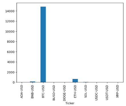
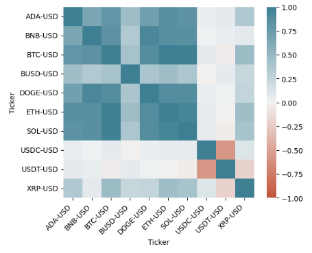
- Plotting the correlation matrix
corr = data['Adj Close'].corr()
ax = sns.heatmap(
    corr,
    vmin=-1, vmax=1, center=0,
    cmap=sns.diverging_palette(20, 220, n=200),
    square=True
)
ax.set_xticklabels(
    ax.get_xticklabels(),
    rotation=45,
    horizontalalignment='right'
);
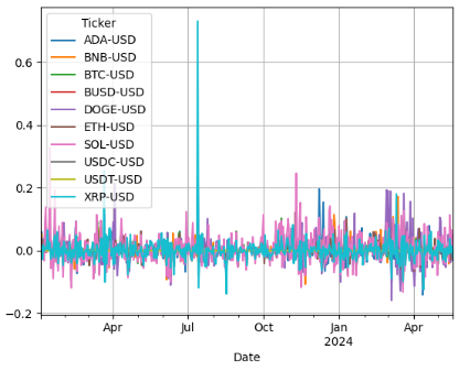
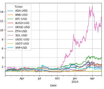
- Plotting daily and cumulative returns
# daily return:
daily_returns = data['Adj Close'].pct_change()

# calculate cumluative return
cum_returns = np.exp(np.log1p(daily_returns).cumsum())
daily_returns.plot() plt.grid()
cum_returns.plot()
plt.grid()
- Let’s implement the simple MPT for Crypto by simulating N_iterations = 150000 portfolios with Monte Carlo, viz.
import matplotlib.pyplot as plt
#calculate percentage change between the current and a prior element - it will be daily returns
daily_returns = data['Adj Close'].pct_change()
num_assets = len(daily_returns.columns)

#calculate covariance matrix
cov_matrix = (daily_returns.cov())*365 # multiply by days in year to get annual covariance

# run optimization of portfolio weights
dict_portfolios = {"portfolio_std":[],"portfolio_returns":[],"weights":[], "sharpe_ratio":[]}
for i in range(N_iterations):

    #get random weights and calculate returns and variance
    weights = np.random.random(num_assets)
    weights = weights/np.sum(weights)
    expected_portfolio_return = np.sum(daily_returns.mean()*weights)
    expected_portfolio_variance = np.dot(weights.T,np.dot(cov_matrix,weights))
    sharpe_ratio = expected_portfolio_return / np.sqrt(expected_portfolio_variance)

    # collect all portfolios in the dictionary
    dict_portfolios['portfolio_std'].append(np.sqrt(expected_portfolio_variance)) # get standard deviation instead of variance
    dict_portfolios['portfolio_returns'].append(expected_portfolio_return)
    dict_portfolios['weights'].append(weights)
    dict_portfolios['sharpe_ratio'].append(sharpe_ratio)

simulated_portfolios=pd.DataFrame(dict_portfolios)

# Plot returns vs. standard deviation to find optimal portfolio (efficient frontier)
simulated_portfolios.plot.scatter(x='portfolio_std', y='portfolio_returns', marker='o', s=10, alpha=0.3, grid=True, figsize=[10,10])
max_sharpe_ratio = simulated_portfolios.query('sharpe_ratio == sharpe_ratio.max()')

# red dot for max sharpe ratio
plt.plot(max_sharpe_ratio['portfolio_std'],max_sharpe_ratio['portfolio_returns'],'ro',markersize=20)
plt.ylabel('Mean daily returns')
plt.xlabel('Annual volatility (standard deviation)')
plt.show()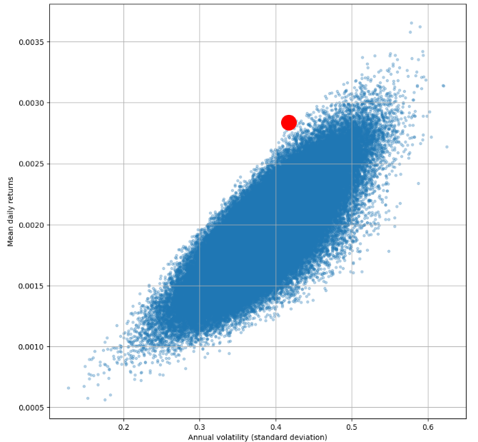
- Checking the portfolio weights
dictionary_of_weights = {}
for i in range(len(daily_returns.columns)):
    dictionary_of_weights [daily_returns.columns[i]] = max_sharpe_ratio['weights'].values[0][i]
print('max sharpe ratio: \n')
efficient_frontier = pd.DataFrame.from_dict(dictionary_of_weights, orient='index').reset_index()
efficient_frontier.columns = ['crypto pair','weights']
display(efficient_frontier)

crypto pair weights
0 ADA-USD 0.028841
1 BNB-USD 0.045777
2 BTC-USD 0.270432
3 BUSD-USD 0.096357
4 DOGE-USD 0.007903
5 ETH-USD 0.022292
6 SOL-USD 0.280154
7 USDC-USD 0.125300
8 USDT-USD 0.103320
9 XRP-USD 0.019625- Creating a pie chart of the above weights
labels = efficient_frontier['crypto pair'][0],efficient_frontier['crypto pair'][1],efficient_frontier['crypto pair'][2],efficient_frontier['crypto pair'][3],efficient_frontier['crypto pair'][4],efficient_frontier['crypto pair'][5],efficient_frontier['crypto pair'][6],efficient_frontier['crypto pair'][7],efficient_frontier['crypto pair'][8],efficient_frontier['crypto pair'][9]
print (labels)
sizes = [efficient_frontier['weights'][0],efficient_frontier['weights'][1],efficient_frontier['weights'][2],efficient_frontier['weights'][3],efficient_frontier['weights'][4],efficient_frontier['weights'][5],efficient_frontier['weights'][6],efficient_frontier['weights'][7],efficient_frontier['weights'][8],efficient_frontier['weights'][9]]
print (sizes)
fig, ax = plt.subplots()
ax.pie(sizes, labels=labels, autopct='%1.1f%%')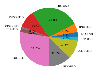
- This is the most efficient allocation that offers the highest return per unit of risk.
Conclusions
- Using the simple MPT for Crypto, we have created a diverse crypto portfolio and evaluated its performance.
- The max Sharpe portfolio yields portfolio_std=0.440951 and portfolio_returns=0.00303 with sharpe_ratio=0.006871 based on mean daily returns and annual volatility (standard deviation).
- The max Sharpe portfolio is expected to offer the max return per unit of risk, while the minimum volatility portfolio is, in fact, the most optimal portfolio with the lowest amount of risk.
- Top 2 assets to include in this portfolio are SOL-USD (28%) and BTC-USD (27%).
Explore More
- Dividend-NG-BTC Diversify Big Tech
- Joint Analysis of Bitcoin, Gold and Crude Oil Prices
- DOGE-INR Price Prediction Backtesting
- BTC-USD Freefall vs FB/Meta Prophet 2022–23 Predictions
- USDTUSD | Tether USD Analysis
- BTC-USD Price Prediction with LSTM
- Bear vs. Bull Portfolio Risk/Return Optimization QC Analysis
References
- Modern portfolio theory for Crypto (simple)
- One of the most important key indicators in the cryptomarket
- The Role of Crypto in a Portfolio
- Using Modern Portfolio Theory and How to Build a Crypto Portfolio
- The Importance of Regularly Optimizing a Crypto Portfolio
- Cryptocurrency portfolio Sharpe ratio optimization
- Analyzing Portfolio Optimization in Cryptocurrency Markets: A Comparative Study of Short-Term Investment Strategies Using Hourly Data Approach
- Portfolio optimization: from the highest Sharpe Ratio to minimum volatility
- Starter: PyPortfolioOpt Stock Prices f9168fca-4


