
Strategic Asset Allocation (SAA) & Portfolio Optimization (PO): Go-To’s for Quants

- This paper represents an in-depth analysis of the Strategic Asset Allocation (SAA) and multi-criteria Portfolio Optimization (PO) methods as a well structured collection of implemented and tested quant trading algorithms in Python.
- The SAA process aims to monitor that the portfolio meets the long-term return and risk targets.
- The PO process selects the best possible combination of investment portfolio assets and their weights.
- The primary goal of both processes is to maximize return while minimizing risk.
Data Science in SAA/PO
- Data science plays a pivotal role in optimizing portfolios and and managing various types of financial risks, including market risk, credit risk, and operational risk.
AI for Quant Trading (AI4QT):
- The objective of AI4QT is to develop a holistic SAA framework by incorporating AI-powered data science [5] into risk-adjusted portfolio optimization (PO) strategies [6,9].
- The idea is take on board key features of the recently released PythonFinanceAI [1–4]. This is a standalone repository that provides insights into various fintech solutions [5, 8], ranging from basics of financial analysis [11] to advanced investment portfolio management algorithms such as Alpha Research and Smart Beta PO.
Algo-Trading Strategies
- This article seeks to provide an in-depth understanding of momentum and breakout trading strategies. These two popular strategies are both dependent on technical analysis.
- Momentum trading involves making investment decisions based on the current market trend.
- Breakout trading is a strategy where investors buy a security when its price moves outside a defined support or resistance level with increased volume.
Fundamentals vs. Technicals
- Fundamental analysis attempts to identify stocks offering strong growth potential at a good price by examining the underlying company’s financial health.
- Technical analysis, on the other hand, looks for statistical patterns on stock charts that might predict future price moves.
- Our goal is to find out how quants can use these two stock-picking strategies together.
Altman Z-Score
- Typically, fundamental analysis is used to assess a company’s value. Here we will provide the Altman Z-score [12] that estimates the likelihood of a company’s bankruptcy.
Let’s delve into the specifics of the aforementioned fintech projects and algorithms.
Alpha Research & Factor Modeling (Portfolio 1)
- In this section, the focus is on the Alpha Research and Factor Modeling strategy (cf. [7, 10]), viz.
- Build a statistical risk model using PCA along with 20 alpha factors.
- Evaluate the factors using factor-weighted returns, quantile analysis, and Sharpe ratio.
- Multiple PO using the risk model and factors.
Scope
- Part 1: Fetching Stock Data and Getting Returns; Part 2: Statistical Risk Model; Part 3: Create Alpha Factors; Part 4: Evaluate Alpha Factors.
- Let’s consider the 5Y Portfolio 1 of 43 stocks
ticker_list = [
    'AAPL', 'ABBV', 'AMGN', 'AMZN', 'AXP', 'BA', 'BIIB', 'BMY', 'CAT', 'CMCSA', 'CSCO', 'CVX', 'DD', 'DIS', 'F', 'GE', 'GILD', 'GM', 'GOOGL',
    'GS', 'HD', 'HON', 'IBM', 'INTC', 'JCI', 'JNJ', 'JPM', 'KO', 'MCD', 'META', 'MMM', 'MRK', 'MSFT', 'PEP', 'PFE', 'PG', 'T', 'TSLA', 'UNH', 'V',
    'VZ', 'WMT', 'XOM'
]

years = 5
year_end = 2024- Importing the necessary libraries and preparing the input data
# Import necessary libraries
import yfinance as yf
import pandas as pd
from datetime import datetime, timedelta
import numpy as np
import json
import matplotlib.pyplot as plt

Fetching Stock Data and Getting Returns
def fetch_stock_data(ticker_list, years=5, year_end=None):
    if year_end is None:
        year_end = datetime.now().year

    end_date = datetime(year_end, 12, 31)
    start_date = end_date - timedelta(days=years * 365)

    close_data_df = pd.DataFrame()
    open_data_df = pd.DataFrame()

    for ticker in ticker_list:
        stock = yf.Ticker(ticker)
        hist_data = stock.history(period='1d', start=start_date, end=end_date)

        # Close Data
        close_data = hist_data['Close'].rename(ticker)
        close_data_df = pd.merge(close_data_df, pd.DataFrame(close_data), left_index=True, right_index=True, how='outer')

        # Open Data
        open_data = hist_data['Open'].rename(ticker)
        open_data_df = pd.merge(open_data_df, pd.DataFrame(open_data), left_index=True, right_index=True, how='outer')

    return close_data_df, open_data_df

close, open = fetch_stock_data(ticker_list, years, year_end)

close.tail()

AAPL ABBV AMGN AMZN AXP BA BIIB BMY CAT CMCSA ... PEP PFE PG T TSLA UNH V VZ WMT XOM
Date
2024-06-14 00:00:00-04:00 212.490005 168.589996 298.619995 183.660004 224.820007 177.270004 231.690002 41.200001 321.470001 37.439999 ... 163.809998 27.530001 166.789993 17.639999 178.009995 495.019989 270.660004 39.669998 67.019997 109.110001
2024-06-17 00:00:00-04:00 216.669998 169.679993 303.279999 184.059998 228.270004 178.389999 226.460007 40.970001 322.399994 37.310001 ... 166.139999 26.980000 167.500000 17.670000 187.440002 489.230011 271.170013 39.459999 67.419998 108.360001
2024-06-18 00:00:00-04:00 214.289993 171.360001 305.989990 182.809998 229.309998 174.990005 223.649994 40.810001 325.140015 36.900002 ... 166.479996 27.410000 168.559998 18.049999 184.860001 481.049988 273.619995 40.080002 67.599998 109.379997
2024-06-20 00:00:00-04:00 209.679993 172.130005 309.890015 186.100006 230.210007 176.300003 225.580002 41.040001 329.130005 37.849998 ... 166.679993 27.740000 167.669998 18.110001 181.570007 484.519989 276.820007 40.240002 68.010002 111.739998
2024-06-21 00:00:00-04:00 207.490005 170.389999 308.160004 189.080002 230.380005 176.559998 224.000000 41.930000 327.839996 38.480000 ... 167.279999 27.740000 168.259995 18.400000 183.009995 482.589996 275.220001 40.240002 67.910004 110.760002
5 rows × 43 columns

close.shape
(1125, 43)

close.info()

<class 'pandas.core.frame.DataFrame'>
DatetimeIndex: 1125 entries, 2020-01-02 00:00:00-05:00 to 2024-06-21 00:00:00-04:00
Data columns (total 43 columns):
 #   Column  Non-Null Count  Dtype
---  ------  --------------  -----
 0   AAPL    1125 non-null   float64
 1   ABBV    1125 non-null   float64
 2   AMGN    1125 non-null   float64
 3   AMZN    1125 non-null   float64
 4   AXP     1125 non-null   float64
 5   BA      1125 non-null   float64
 6   BIIB    1125 non-null   float64
 7   BMY     1125 non-null   float64
 8   CAT     1125 non-null   float64
 9   CMCSA   1125 non-null   float64
 10  CSCO    1125 non-null   float64
 11  CVX     1125 non-null   float64
 12  DD      1125 non-null   float64
 13  DIS     1125 non-null   float64
 14  F       1125 non-null   float64
 15  GE      1125 non-null   float64
 16  GILD    1125 non-null   float64
 17  GM      1125 non-null   float64
 18  GOOGL   1125 non-null   float64
 19  GS      1125 non-null   float64
 20  HD      1125 non-null   float64
 21  HON     1125 non-null   float64
 22  IBM     1125 non-null   float64
 23  INTC    1125 non-null   float64
 24  JCI     1125 non-null   float64
 25  JNJ     1125 non-null   float64
 26  JPM     1125 non-null   float64
 27  KO      1125 non-null   float64
 28  MCD     1125 non-null   float64
 29  META    1125 non-null   float64
 30  MMM     1125 non-null   float64
 31  MRK     1125 non-null   float64
 32  MSFT    1125 non-null   float64
 33  PEP     1125 non-null   float64
 34  PFE     1125 non-null   float64
 35  PG      1125 non-null   float64
 36  T       1125 non-null   float64
 37  TSLA    1125 non-null   float64
 38  UNH     1125 non-null   float64
 39  V       1125 non-null   float64
 40  VZ      1125 non-null   float64
 41  WMT     1125 non-null   float64
 42  XOM     1125 non-null   float64
dtypes: float64(43)
memory usage: 386.7 KB- Examining the descriptive statistics summary of the dataset
close.describe().T

count mean std min 25% 50% 75% max
AAPL 1125.0 143.658611 34.734293 54.632896 123.990799 146.971649 171.161026 216.669998
ABBV 1125.0 120.252841 31.394200 53.663055 93.122742 130.147095 144.791183 180.415100
AMGN 1125.0 229.201625 30.390542 159.913116 208.148529 222.399857 245.879562 319.771271
AMZN 1125.0 141.189915 28.669234 81.820000 116.750000 148.023499 164.868500 189.500000
AXP 1125.0 150.053098 36.689715 64.962784 127.278458 153.474594 167.936493 243.080002
BA 1125.0 199.101303 41.000993 95.010002 173.160004 202.720001 218.759995 345.395020
BIIB 1125.0 264.431298 40.002559 187.539993 231.990005 267.869995 286.540009 414.709991
BMY 1125.0 58.363579 7.720472 40.207870 52.710373 57.102249 64.020714 76.548782
CAT 1125.0 207.083070 62.089769 83.515442 172.211151 203.556000 236.764145 377.922363
CMCSA 1125.0 41.974927 6.296697 27.474335 37.743309 41.433960 46.057053 57.373844
CSCO 1125.0 45.861873 5.738260 29.084276 41.383766 46.999535 50.200222 59.220711
CVX 1125.0 120.667475 36.004832 44.864265 87.971695 134.733536 153.243607 176.953262
DD 1125.0 64.932338 11.107107 26.226181 56.228531 68.340065 73.100937 82.160004
DIS 1125.0 124.724984 33.161822 79.062325 97.129997 113.849998 149.622360 201.254089
F 1125.0 10.669939 3.193563 3.364042 9.495123 11.201049 12.310000 21.238628
GE 1125.0 67.139188 30.726982 26.821478 47.380741 61.730171 80.237434 168.860001
GILD 1125.0 64.485216 8.982150 48.918766 57.292091 62.327827 73.114235 85.358162
GM 1125.0 39.789857 10.409134 16.454935 32.726471 37.865936 47.570000 64.389725
GOOGL 1125.0 112.715794 28.157881 52.646080 89.788452 114.440659 135.842102 179.630005
GS 1125.0 303.479342 73.462022 121.462883 270.750275 317.004181 350.596802 467.580383
HD 1125.0 287.946219 46.524254 137.325714 258.115295 290.264862 315.013367 392.471649
HON 1125.0 184.879189 23.944280 95.141182 175.067902 190.931870 201.240326 220.703552
IBM 1125.0 122.849117 23.973442 73.761368 105.327614 119.168266 131.599976 195.835968
INTC 1125.0 42.294133 9.593616 23.974878 33.875050 44.011238 49.978661 62.477165
JCI 1125.0 54.227994 12.665147 21.432339 46.875332 56.875942 63.770000 76.871490
JNJ 1125.0 150.426623 12.724748 98.888367 145.279999 153.009399 158.975784 174.296173
JPM 1125.0 131.705269 28.884633 69.640205 111.258682 134.498169 147.201843 204.789993
KO 1125.0 53.109379 6.713766 32.919655 48.319462 55.395565 58.796181 63.656071
MCD 1125.0 234.139605 37.086671 124.335892 204.344177 237.010330 263.060455 296.902130
META 1125.0 271.613339 95.444213 88.727669 201.665588 268.388489 328.095795 526.816956
MMM 1125.0 104.554440 20.317660 68.398048 87.095383 104.484344 120.384705 146.007172
MRK 1125.0 86.375625 20.211091 55.622543 68.933578 78.446602 104.073280 131.165314
MSFT 1125.0 273.887771 70.907046 130.375595 224.182755 265.359100 321.913879 449.779999
PEP 1125.0 150.520650 21.307595 92.089531 129.536469 157.412201 167.235062 188.991516
PFE 1125.0 35.864667 7.338801 22.702326 29.745178 34.496193 42.067959 55.076660
PG 1125.0 135.360503 15.846908 87.905472 125.435829 135.991638 147.639648 168.559998
T 1125.0 16.692364 1.474788 12.776750 15.869843 16.803026 17.472309 21.093868
TSLA 1125.0 206.531430 81.738779 24.081333 166.660004 216.419998 258.079987 409.970001
UNH 1125.0 422.687371 91.189455 183.182266 333.794434 462.890991 496.851379 546.607117
V 1125.0 217.368442 27.959699 131.732117 198.659409 213.533295 230.491501 289.833618
VZ 1125.0 41.765110 5.625551 29.680738 36.542049 44.023743 46.539070 50.483551
WMT 1125.0 46.695827 6.333629 32.341011 43.098869 45.827610 49.881126 68.010002
XOM 1125.0 73.847216 29.364404 25.440153 49.019825 76.831482 102.509506 121.215431- Plotting the volatility (STD) column
yy=close.describe().T

plt.figure(figsize=(22,6))
plt.bar(ticker_list,yy['std'])
plt.title('Volatility (STD)')
plt.grid()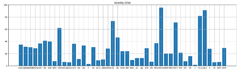
- Calculating and plotting the price range as the Max/Min ratio
yy=close.describe().T

plt.figure(figsize=(22,6))
plt.bar(ticker_list,yy['max']/yy['min'])
plt.title('Max/Min Price Ratio')
plt.grid()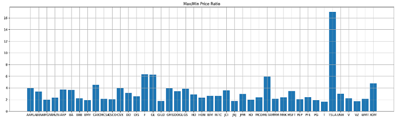
- Calculating the stock normalize price or cumulative return 2023–2024
def plot_data2(df,stocks,title='Stock Prices',ylabel="Stock Price",start='2023-01-03', end ='2024-06-21'):

    """ This function creates a plot of adjusted close stock prices
    inputs:
    df - dataframe
    title - plot title
    stocks - the stock symbols of each company
    ylabel - y axis label
    y - horizontal line(integer)
    output: the plot of adjusted close stock prices
    """
    df_new = df[start:end]
    ax = df_new.plot(title=title, figsize=(20,14), ax = None)
    ax.set_xlabel("Date")
    ax.set_ylabel(ylabel)
    ax.legend(stocks, loc='upper left')
    plt.grid()
    plt.show()

# create function that normalizes the data
def normalize_data(df):
    """
    This function normalizes the stock prices using the first row of the dataframe
    input - stock data
    output - normalized stock data
    """
    return df/df.iloc[0,:]

stocks = ticker_list

plot_data2(normalize_data(close),stocks,title = "Normalized Stock Prices", ylabel = 'Cumulative Return')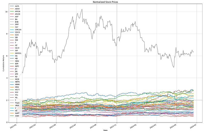
- Calculating the stock daily returns
def generate_returns(prices, shift):
    return_prices = prices.pct_change(shift).iloc[shift:, :]
    return return_prices

returns = generate_returns(close, 1)
returns.tail()

AAPL ABBV AMGN AMZN AXP BA BIIB BMY CAT CMCSA ... PEP PFE PG T TSLA UNH V VZ WMT XOM
Date
2024-06-14 00:00:00-04:00 -0.008168 0.012188 0.000402 -0.000925 0.011837 -0.018982 -0.009194 -0.006750 -0.014983 -0.003725 ... 0.002939 -0.004340 0.002283 -0.001698 -0.024442 -0.000362 -0.001954 -0.002765 0.004798 -0.008451
2024-06-17 00:00:00-04:00 0.019671 0.006465 0.015605 0.002178 0.015346 0.006318 -0.022573 -0.005583 0.002893 -0.003472 ... 0.014224 -0.019978 0.004257 0.001701 0.052975 -0.011696 0.001884 -0.005294 0.005968 -0.006874
2024-06-18 00:00:00-04:00 -0.010984 0.009901 0.008936 -0.006791 0.004556 -0.019059 -0.012408 -0.003905 0.008499 -0.010989 ... 0.002046 0.015938 0.006328 0.021505 -0.013764 -0.016720 0.009035 0.015712 0.002670 0.009413
2024-06-20 00:00:00-04:00 -0.021513 0.004493 0.012746 0.017997 0.003925 0.007486 0.008630 0.005636 0.012272 0.025745 ... 0.001201 0.012039 -0.005280 0.003324 -0.017797 0.007213 0.011695 0.003992 0.006065 0.021576
2024-06-21 00:00:00-04:00 -0.010444 -0.010109 -0.005583 0.016013 0.000738 0.001475 -0.007004 0.021686 -0.003919 0.016645 ... 0.003600 0.000000 0.003519 0.016013 0.007931 -0.003983 -0.005780 0.000000 -0.001470 -0.008770
5 rows × 43 columns- Plotting the AAPL daily return as an example
returns['AAPL'].plot(figsize=(12,6))
plt.grid()
plt.title('AAPL Returns')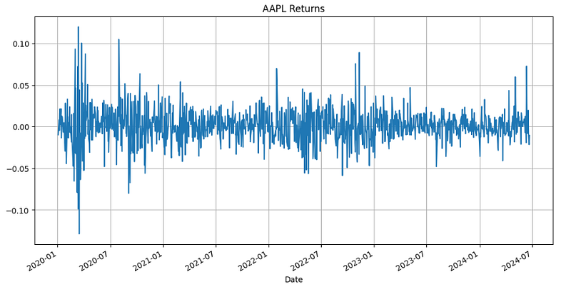
- Calculating and plotting the kurtosis of daily returns
plt.figure(figsize=(12, 6))
retkurt=returns.kurt()
retkurt.plot.bar()
plt.grid()
plt.title('Kurtosis')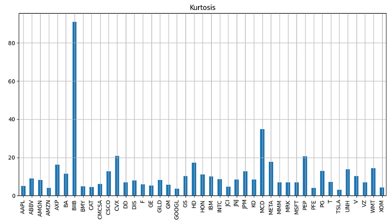
- Calculating and plotting the skewness of daily returns
plt.figure(figsize=(12, 6))
retkurt=returns.skew()
retkurt.plot.bar()
plt.grid()
plt.title('Skewness')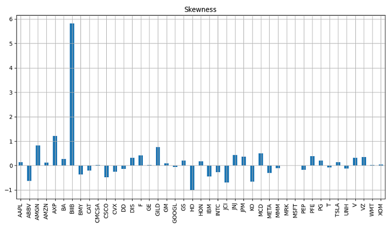
- Creating the Statistical Risk Model
- Performing SVD PCA of daily return in terms of 20 factor exposures
# Fit PCA
from sklearn.decomposition import PCA

def fit_pca(returns, num_factor_exposures, svd_solver):
    pca = PCA(n_components=num_factor_exposures, svd_solver=svd_solver)
    return pca.fit(returns)

num_factor_exposures = 20
pca = fit_pca(returns, num_factor_exposures, 'full')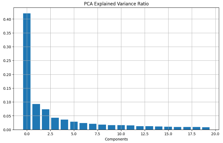
2. Calculating the factor betas in terms of PCA vs factor exposures
#Factor Betas
def factor_betas(pca, factor_beta_indices, factor_beta_columns):
    factor_betas = pd.DataFrame(pca.components_.T, factor_beta_indices, factor_beta_columns)

    return factor_betas

risk_model = {}
risk_model['factor_betas'] = factor_betas(pca, returns.columns.values, np.arange(num_factor_exposures))- Plotting the factor betas
risk_model['factor_betas'].plot.bar(figsize=(18,6))
plt.grid()
plt.title('Factor Betas')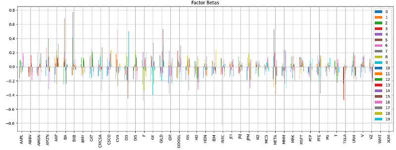
3. Calculating and plotting the factor returns
# Factor Returns
def factor_returns(pca, returns, factor_return_indices, factor_return_columns):
    factor_returns = pd.DataFrame(pca.transform(returns), factor_return_indices, factor_return_columns)
    return factor_returns

risk_model['factor_returns'] = factor_returns(
    pca,
    returns,
    returns.index,
    np.arange(num_factor_exposures))

risk_model['factor_returns'].plot(figsize=(20,6))
plt.grid()
plt.title('Factor Returns')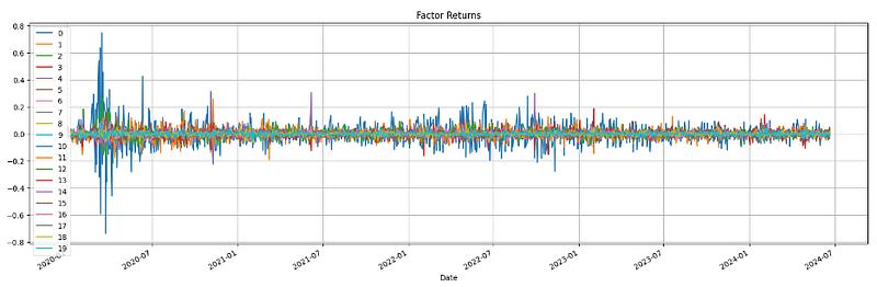
4. Calculating and plotting the factor covariance matrix
# Factor Covariance Matrix
def factor_cov_matrix(factor_returns, ann_factor):
    factor_cov_matrix = np.var(factor_returns, ddof=1)
    factor_cov_matrix = np.diag(factor_cov_matrix) * ann_factor
    return factor_cov_matrix

ann_factor = 252 # Annualization factor
risk_model['factor_cov_matrix'] = factor_cov_matrix(risk_model['factor_returns'], ann_factor)

from matplotlib.pyplot import imshow
import numpy as np
data = risk_model['factor_cov_matrix']
imshow(np.asarray(data),vmin=0, vmax=1, cmap='jet')
plt.colorbar()
plt.title('Factor Covariance Matrix')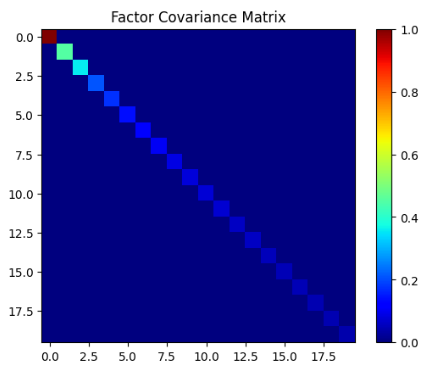
5. Calculating and plotting the Idiosyncratic Variance Matrix
# Idiosyncratic Variance Matrix
def idiosyncratic_var_matrix(returns, factor_returns, factor_betas, ann_factor):
    dot_product = np.dot(factor_returns, factor_betas.T)
    common_return = pd.DataFrame(dot_product, returns.index, returns.columns)
    residual_return = returns - common_return

    idiosyncratic_var_matrix = pd.DataFrame(np.diag(np.var(residual_return)) * ann_factor, returns.columns, returns.columns)

    return idiosyncratic_var_matrix

risk_model['idiosyncratic_var_matrix'] = idiosyncratic_var_matrix(returns, risk_model['factor_returns'], risk_model['factor_betas'], ann_factor)

from matplotlib.pyplot import imshow
import numpy as np
data = risk_model['idiosyncratic_var_matrix']
imshow(np.asarray(data),cmap='jet')
plt.colorbar()
plt.title('Idiosyncratic Variance Matrix')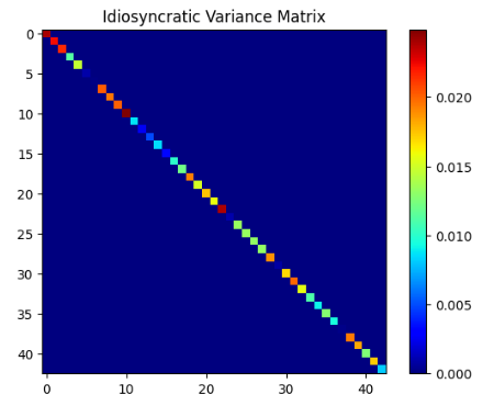
6. Calculating and plotting the Idiosyncratic Variance Vector
# Idiosyncratic Variance Vector
def idiosyncratic_var_vector(returns, idiosyncratic_var_matrix):
    idiosyncratic_var_vector = pd.DataFrame(np.diagonal(idiosyncratic_var_matrix), returns.columns)

    return idiosyncratic_var_vector

risk_model['idiosyncratic_var_vector'] = idiosyncratic_var_vector(returns, risk_model['idiosyncratic_var_matrix'])

from matplotlib.pyplot import imshow
import numpy as np
data = risk_model['idiosyncratic_var_vector']

risk_model['idiosyncratic_var_vector'].plot.bar(figsize=(18,6))
plt.grid()
plt.title('Idiosyncratic Variance Vector')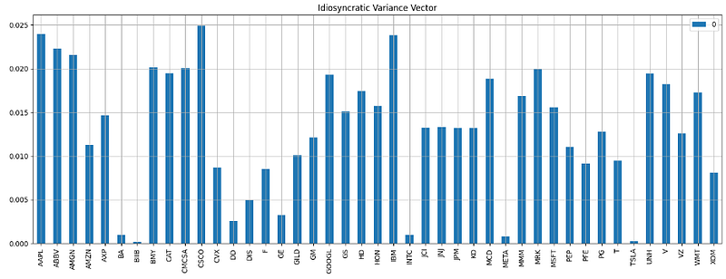
7. Predicting the expected portfolio risk using the above Risk Model
# Predict using the Risk Model
def predict_portfolio_risk(factor_betas, factor_cov_matrix, idiosyncratic_var_matrix, weights):
    form_break_01 = np.dot(np.dot(factor_betas, factor_cov_matrix), factor_betas.T) + idiosyncratic_var_matrix # (BFB.T + S)
    form_break_02 = np.dot(np.dot(weights.T, form_break_01), weights) # (X.T(form_break_01)X)

    predicted_portfolio_risk = np.sqrt(form_break_02)

    return predicted_portfolio_risk[0][0]

all_weights = pd.DataFrame(np.repeat(1/len(ticker_list), len(ticker_list)), ticker_list)

predict_portfolio_risk(
    risk_model['factor_betas'],
    risk_model['factor_cov_matrix'],
    risk_model['idiosyncratic_var_matrix'],
    all_weights)

0.2090265849547022- Creating the Alpha Factors
#Part 3: Create Alpha Factors
# Function to fetch sector information for a list of tickers
def fetch_sector_data(ticker_list):
    sector = {}
    for ticker in ticker_list:
        tickerdata = yf.Ticker(ticker)
        sector[ticker] = tickerdata.info.get('sector', 'Unknown')
    return sector

sectors_data = fetch_sector_data(ticker_list)
sectors_series = pd.Series(sectors_data)

print(sectors_series)

AAPL                 Technology
ABBV                 Healthcare
AMGN                 Healthcare
AMZN          Consumer Cyclical
AXP          Financial Services
BA                  Industrials
BIIB                 Healthcare
BMY                  Healthcare
CAT                 Industrials
CMCSA    Communication Services
CSCO                 Technology
CVX                      Energy
DD              Basic Materials
DIS      Communication Services
F             Consumer Cyclical
GE                  Industrials
GILD                 Healthcare
GM            Consumer Cyclical
GOOGL    Communication Services
GS           Financial Services
HD            Consumer Cyclical
HON                 Industrials
IBM                  Technology
INTC                 Technology
JCI                 Industrials
JNJ                  Healthcare
JPM          Financial Services
KO           Consumer Defensive
MCD           Consumer Cyclical
META     Communication Services
MMM                 Industrials
MRK                  Healthcare
MSFT                 Technology
PEP          Consumer Defensive
PFE                  Healthcare
PG           Consumer Defensive
T        Communication Services
TSLA          Consumer Cyclical
UNH                  Healthcare
V            Financial Services
VZ       Communication Services
WMT          Consumer Defensive
XOM                      Energy
dtype: object- Plotting the Histogram of Industry Sectors involved
plt.figure(figsize=(16,6))
sectors_series.hist()
plt.title('Histogram of Industry Sectors')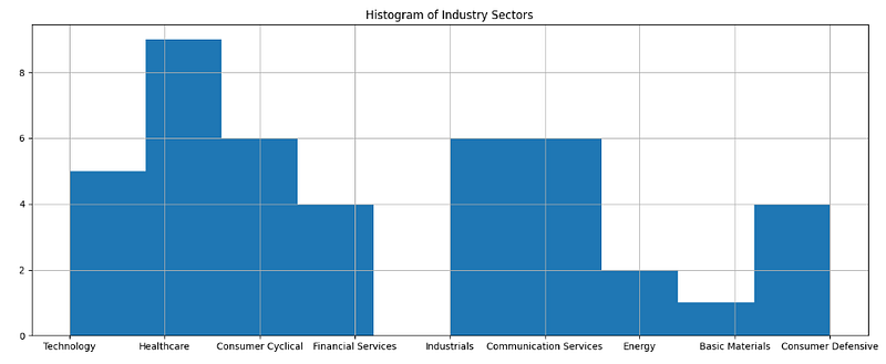
- Implementing the Mean_Reversion_5Day_Sector_Neutral factor
# Mean Reversion 5 Day Sector Neutral Factor
# Auxiliary function to calculate z-scores
def calculate_z_scores(demeaned):
    # Adding a small value to the standard deviation to avoid division by zero
    epsilon = 1e-7
    demeaned_std_aligned = demeaned.std(axis=1).to_frame(name='std')
    demeaned_std_aligned = pd.concat([demeaned_std_aligned] * demeaned.shape[1], axis=1)
    demeaned_std_aligned.columns = demeaned.columns
    demeaned_std_aligned += epsilon

    # Calculating z-scores
    demeaned_mean_aligned = demeaned.mean(axis=1).to_frame(name='mean')
    demeaned_mean_aligned = pd.concat([demeaned_mean_aligned] * demeaned.shape[1], axis=1)
    demeaned_mean_aligned.columns = demeaned.columns
    z_scored = (demeaned - demeaned_mean_aligned) / demeaned_std_aligned

    return z_scored

# Function for 5-day sector neutral mean reversion
def calculate_mean_reversion_5day_sector_neutral(returns, sectors):
    # Aligning sectors with the return columns
    aligned_sectors = sectors_series.reindex(returns.columns)

    # Subtracting the sector mean from each return
    sector_means = returns.groupby(aligned_sectors, axis=1).transform('mean')
    demeaned = - returns.sub(sector_means)

    # Normalizing the results
    demeaned = demeaned.rank(axis=1)
    z_scored = calculate_z_scores(demeaned)

    # Converting to long format
    z_scored_long = z_scored.stack().reset_index()
    z_scored_long.columns = ['Date', 'Ticker', 'Mean_Reversion_5Day_Sector_Neutral']

    return z_scored_long

# Calculating 5-day returns
returns_5d = generate_returns(close, 5)

# Applying the function
mean_reversion_5day_sector_neutral = calculate_mean_reversion_5day_sector_neutral(returns_5d, sectors_series)

mean_reversion_5day_sector_neutral.set_index(['Date', 'Ticker'])

Mean_Reversion_5Day_Sector_Neutral
Date Ticker
2020-01-09 00:00:00-05:00 AAPL -1.433516
ABBV -0.318559
AMGN 0.557478
AMZN 0.955677
AXP -0.238919
... ... ...
2024-06-21 00:00:00-04:00 UNH 1.513156
V 0.398199
VZ 0.637118
WMT -0.079640
XOM 0.477839
48160 rows × 1 columns- Implementing the Mean_Reversion_5Day_Sector_Neutral_Smoothed factor
# Mean Reversion 5 Day Sector Neutral Smoothed Factor
# Function for smoothed 5-day sector neutral mean reversion
def calculate_mean_reversion_5day_sector_neutral_smoothed(factor_long):
    # Reconverting to wide format for smoothing
    factor_wide = factor_long.pivot(index='Date', columns='Ticker', values='Mean_Reversion_5Day_Sector_Neutral')

    # Smoothing using simple moving average
    smoothed = factor_wide.rolling(window=5).mean()

    # Normalizing the results again
    smoothed = smoothed.rank(axis=1)
    z_scored = calculate_z_scores(smoothed)

    # Converting to long format
    z_scored_long = z_scored.stack().reset_index()
    z_scored_long.columns = ['Date', 'Ticker', 'Mean_Reversion_5Day_Sector_Neutral_Smoothed']

    return z_scored_long

mean_reversion_5day_sector_neutral_smoothed = calculate_mean_reversion_5day_sector_neutral_smoothed(mean_reversion_5day_sector_neutral.reset_index())

mean_reversion_5day_sector_neutral_smoothed.set_index(['Date', 'Ticker'])

Mean_Reversion_5Day_Sector_Neutral_Smoothed
Date Ticker
2020-01-15 00:00:00-05:00 AAPL -1.433733
ABBV 0.318607
AMGN 0.438085
AMZN 1.593036
AXP -0.557563
... ... ...
2024-06-21 00:00:00-04:00 UNH 0.796398
V 0.398199
VZ 0.557478
WMT -1.114957
XOM 0.637118
47988 rows × 1 columns- Implementing the Sum_Overnight_Sentiment_5Day factor
# Overnight Sentiment Factor
# Function to calculate overnight returns
def calculate_overnight_returns(open_prices, close_prices):
    # Calculating the return from yesterday's close to today's open
    return (open_prices - close_prices.shift(1)) / close_prices.shift(1)

# Function to calculate trailing overnight returns
def calculate_overnight_sentiment(overnight_returns, window_length):
    # Calculating the rolling sum of overnight returns
    summed = overnight_returns.rolling(window=window_length).sum()

    # Normalizing the results by converting to z-score
    z_scored = calculate_z_scores(summed)

    # Converting back to long format
    z_scored_long = z_scored.stack().reset_index()
    z_scored_long.columns = ['Date', 'Ticker', 'Sum_Overnight_Sentiment_5Day']

    return z_scored_long

# Applying the functions
overnight_returns = calculate_overnight_returns(open, close)
overnight_sentiment = calculate_overnight_sentiment(overnight_returns, window_length=5)

overnight_sentiment.set_index(['Date', 'Ticker'])

Sum_Overnight_Sentiment_5Day
Date Ticker
2020-01-09 00:00:00-05:00 AAPL -0.061856
ABBV -0.349628
AMGN -0.232041
AMZN -0.506176
AXP -0.097025
... ... ...
2024-06-21 00:00:00-04:00 UNH -0.239129
V -0.392243
VZ -0.114173
WMT 0.208194
XOM 1.099303
48160 rows × 1 columns- Implementing the Sum_Overnight_Sentiment_5Day_Smoothed factor
# Overnight Sentiment Smoothed Factor
def calculate_overnight_sentiment_smoothed(overnight_sentiment):
    # Reconverting to wide format for smoothing
    overnight_wide = overnight_sentiment.pivot(index='Date', columns='Ticker', values='Sum_Overnight_Sentiment_5Day')

    # Smoothing using simple moving average
    smoothed = overnight_wide.rolling(window=5).mean()

    # Normalizing the results again
    smoothed = smoothed.rank(axis=1)
    z_scored = calculate_z_scores(smoothed)

    # Converting to long format
    z_scored_long = z_scored.stack().reset_index()
    z_scored_long.columns = ['Date', 'Ticker', 'Sum_Overnight_Sentiment_5Day_Smoothed']

    return z_scored_long

overnight_sentiment_smoothed = calculate_overnight_sentiment_smoothed(overnight_sentiment.reset_index())

overnight_sentiment_smoothed.set_index(['Date', 'Ticker'])

Sum_Overnight_Sentiment_5Day_Smoothed
Date Ticker
2020-01-15 00:00:00-05:00 AAPL 1.035317
ABBV 0.079640
AMGN -0.716758
AMZN 0.398199
AXP 0.477839
... ... ...
2024-06-21 00:00:00-04:00 UNH -0.557478
V 0.000000
VZ 0.637118
WMT 1.114957
XOM 1.433516
47988 rows × 1 columns- Combining all the above Factors into a single DF
# Combine the Factors
from functools import reduce

# Create a list of all dataframes
dataframes = [mean_reversion_5day_sector_neutral,
              mean_reversion_5day_sector_neutral_smoothed,
              overnight_sentiment,
              overnight_sentiment_smoothed]

# Use 'reduce' to merge all dataframes into a single dataframe
all_factors = reduce(lambda left, right: pd.merge(left, right, on=['Date', 'Ticker'], how='inner'), dataframes)

# Readjust 'Date' and 'Ticker' as indices
all_factors = all_factors.set_index(['Date', 'Ticker'])

all_factors['Combined_Factors'] = all_factors.mean(axis=1)

all_factors

Mean_Reversion_5Day_Sector_Neutral Mean_Reversion_5Day_Sector_Neutral_Smoothed Sum_Overnight_Sentiment_5Day Sum_Overnight_Sentiment_5Day_Smoothed Combined_Factors
Date Ticker
2020-01-15 00:00:00-05:00 AAPL -0.955677 -1.433733 0.690153 1.035317 -0.165985
ABBV 0.637118 0.318607 -0.073723 0.079640 0.240410
AMGN 0.000000 0.438085 -0.430507 -0.716758 -0.177295
AMZN 1.513156 1.593036 0.488492 0.398199 0.998221
AXP -0.716758 -0.557563 0.107696 0.477839 -0.172197
... ... ... ... ... ... ...
2024-06-21 00:00:00-04:00 UNH 1.513156 0.796398 -0.239129 -0.557478 0.378237
V 0.398199 0.398199 -0.392243 0.000000 0.101039
VZ 0.637118 0.557478 -0.114173 0.637118 0.429386
WMT -0.079640 -1.114957 0.208194 1.114957 0.032139
XOM 0.477839 0.637118 1.099303 1.433516 0.911944
47988 rows × 5 columns- Evaluating the Alpha Factors
#A. Factor Returns
# Calculate forward returns and align with factor data dates
forward_returns = generate_returns(close, 1).shift(-1).reset_index()
forward_returns = forward_returns.loc[forward_returns['Date'].isin(set(all_factors.reset_index().Date))].set_index('Date')
forward_returns = forward_returns.stack().reset_index()
forward_returns.columns = ['Date', 'Ticker', 'Returns']
forward_returns.set_index(['Date', 'Ticker'], inplace=True)

def calculate_allocation(df):
    df[df < 0] = 0
    return df.groupby(level=0, group_keys=False).apply(lambda x: x / x.sum())

# Calculate allocations and combine with forward returns
allocation = all_factors.copy()
allocation = calculate_allocation(allocation)
strategy_returns = allocation.reset_index().merge(forward_returns.reset_index(), on=['Date', 'Ticker']).set_index(['Date', 'Ticker'])

# Apply allocation weights to returns
strategy_returns.update(strategy_returns.drop(columns='Returns').mul(strategy_returns['Returns'], axis=0))

# Calculate strategy and benchmark returns
mean_returns = strategy_returns[['Returns']].groupby(level=0, group_keys=False).apply(lambda x: x.mean())
strategy_returns = strategy_returns.drop(columns='Returns').groupby(level=0, group_keys=False).apply(lambda x: x.sum())
strategy_returns['Benchmark'] = mean_returns

# Plot cumulative returns
(1 + strategy_returns).cumprod().plot(figsize=(12, 5))
plt.title('Portfolio Cumulative Return')
plt.grid()
plt.show()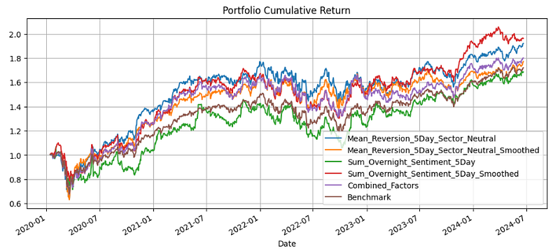
- Correlation Analysis: calculate the correlation matrix for alpha factors
#B. Correlation Analysis
# Calculate the correlation matrix for alpha factors
correlation_matrix = all_factors.corr()
correlation_matrix.style.background_gradient(cmap='RdBu')

                                            Mean_Reversion_5Day_Sector_Neutral Mean_Reversion_5Day_Sector_Neutral_Smoothed Sum_Overnight_Sentiment_5Day Sum_Overnight_Sentiment_5Day_Smoothed Combined_Factors
Mean_Reversion_5Day_Sector_Neutral           1.000000 0.691424 -0.371131 -0.242775 0.523061
Mean_Reversion_5Day_Sector_Neutral_Smoothed  0.691424 1.000000 -0.270885 -0.339575 0.524734
Sum_Overnight_Sentiment_5Day                 -0.371131 -0.270885 1.000000 0.654801 0.491634
Sum_Overnight_Sentiment_5Day_Smoothed        -0.242775 -0.339575 0.654801 1.000000 0.520599
Combined_Factors                             0.523061 0.524734 0.491634 0.520599 1.000000

f = plt.figure(figsize=(12, 10))
plt.matshow(correlation_matrix, fignum=f.number)
cb = plt.colorbar()
cb.ax.tick_params(labelsize=14)
plt.title('Correlation Matrix', fontsize=16);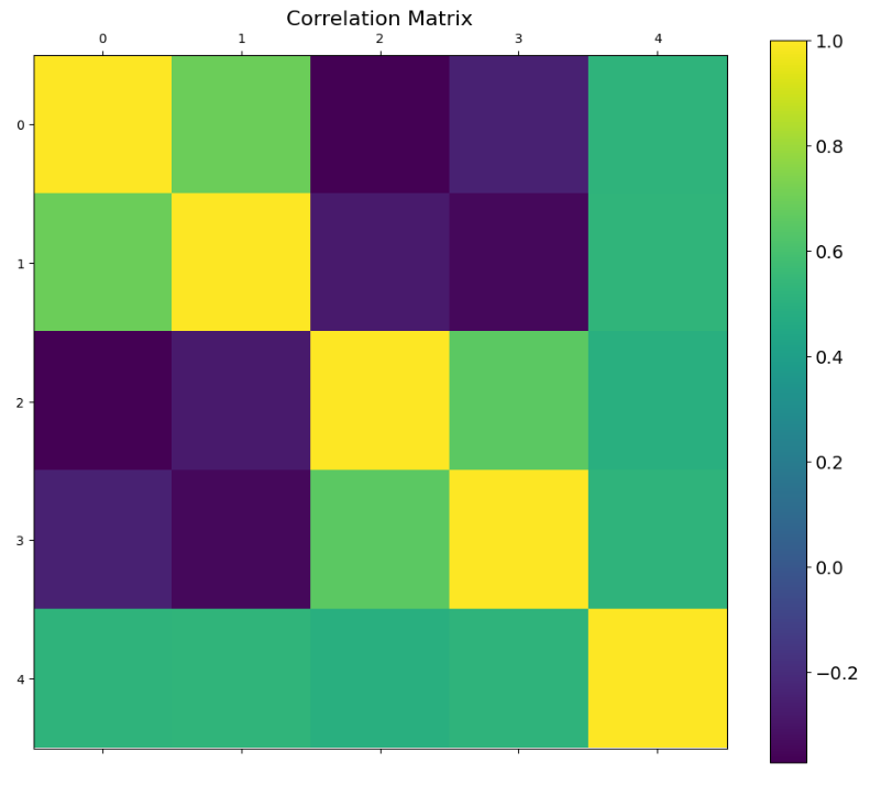
- Explaining the correlation matrix columns 0–4
correlation_matrix.columns
Index(['Mean_Reversion_5Day_Sector_Neutral',
       'Mean_Reversion_5Day_Sector_Neutral_Smoothed',
       'Sum_Overnight_Sentiment_5Day', 'Sum_Overnight_Sentiment_5Day_Smoothed',
       'Combined_Factors'],
dtype='object')- Drawdown Analysis
#C. Drawdown Analysis
# Calculate cumulative returns
cumulative_returns = (1 + strategy_returns).cumprod()

# Drawdown Analysis
peak = cumulative_returns.expanding(min_periods=1).max()
drawdown = (cumulative_returns - peak) / peak

plt.figure(figsize=(8, 4))
plt.barh(drawdown.min().index, drawdown.min(), color='red')
plt.xlabel('Drawdown')
plt.grid()
plt.show()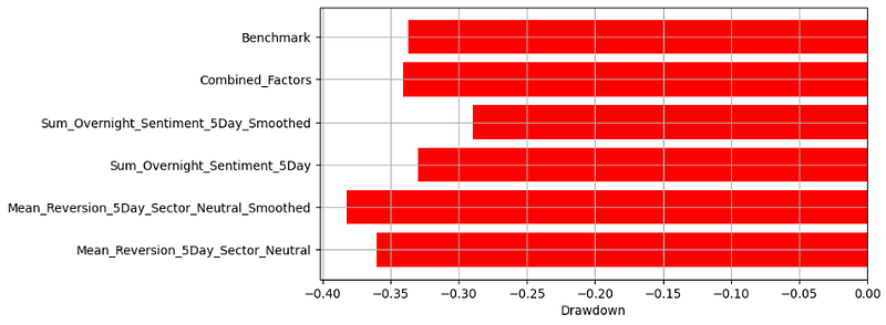
- Calculating the Return/Volatility Ratio
#D. Return to Volatility Ratio
# Calculate annualized return
annualized_return = strategy_returns.mean() * 252

# Calculate annualized volatility
annualized_volatility = strategy_returns.std() * np.sqrt(252)

# Return to volatility ratio
return_to_volatility_ratio = annualized_return / annualized_volatility

plt.figure(figsize=(8, 4))
plt.barh(return_to_volatility_ratio.index, return_to_volatility_ratio, color='darkblue')
plt.xlabel('Return/Volatility Ratio')
plt.grid()
plt.show()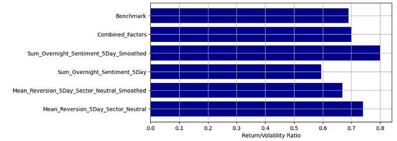
Smart Beta PO (Portfolio 2)
- Let’s explore the application of the Smart Beta strategy in PO, viz. Part 1: Fetching Stock Data; Part 2: Creating Weights for Benchmarks; Part 3: Portfolio Optimization (Smart Beta Strategy).
- Let’s look at the 5Y Portfolio 2 of 10 stocks
# Fetch the data
ticker_list = ['PG', 'JNJ', 'KO', 'MCD', 'MMM', 'IBM', 'PEP', 'T', 'VZ', 'WMT']
years = 5- Importing libraries and fetching the relevant stock data, v.i.
# Import necessary libraries
import yfinance as yf
import pandas as pd
from datetime import datetime, timedelta
import numpy as np
import json
import matplotlib.pyplot as plt

#Part 1: Fetching Stock Data
def fetch_stock_data(ticker_list, years=5):
    end_date = datetime.now()
    start_date = end_date - timedelta(days=years * 365)

    close_data_df = pd.DataFrame()
    volume_data_df = pd.DataFrame()
    dividends_data_df = pd.DataFrame()

    for ticker in ticker_list:
        stock = yf.Ticker(ticker)
        hist_data = stock.history(period='1d', start=start_date, end=end_date)

        # Close Data
        close_data = hist_data['Close'].rename(ticker)
        close_data_df = pd.merge(close_data_df, pd.DataFrame(close_data), left_index=True, right_index=True, how='outer')

        # Volume Data
        volume_data = hist_data['Volume'].rename(ticker)
        volume_data_df = pd.merge(volume_data_df, pd.DataFrame(volume_data), left_index=True, right_index=True, how='outer')

        # Dividends Data
        dividends_data = hist_data['Dividends'].rename(ticker)
        dividends_data_df = pd.merge(dividends_data_df, pd.DataFrame(dividends_data), left_index=True, right_index=True, how='outer')

    return close_data_df, volume_data_df, dividends_data_df


close, volume, dividends = fetch_stock_data(ticker_list, years)
close.tail()

                          PG          JNJ        KO        MCD        MMM          IBM      PEP        T          VZ       WMT
Date
2024-06-14 00:00:00-04:00 166.789993 145.539993 62.549999 253.580002 100.900002 169.210007 163.809998 17.639999 39.669998 67.019997
2024-06-17 00:00:00-04:00 167.500000 145.949997 62.619999 253.509995 100.529999 169.500000 166.139999 17.670000 39.459999 67.419998
2024-06-18 00:00:00-04:00 168.559998 145.649994 62.630001 250.789993 100.769997 170.550003 166.479996 18.049999 40.080002 67.599998
2024-06-20 00:00:00-04:00 167.669998 147.779999 62.180000 253.800003 101.660004 173.919998 166.679993 18.110001 40.240002 68.010002
2024-06-21 00:00:00-04:00 168.259995 148.750000 62.770000 259.390015 102.389999 172.460007 167.279999 18.400000 40.240002 67.910004

close.shape
(1257, 10)

close.info()

<class 'pandas.core.frame.DataFrame'>
DatetimeIndex: 1257 entries, 2019-06-25 00:00:00-04:00 to 2024-06-21 00:00:00-04:00
Data columns (total 10 columns):
 #   Column  Non-Null Count  Dtype
---  ------  --------------  -----
 0   PG      1257 non-null   float64
 1   JNJ     1257 non-null   float64
 2   KO      1257 non-null   float64
 3   MCD     1257 non-null   float64
 4   MMM     1257 non-null   float64
 5   IBM     1257 non-null   float64
 6   PEP     1257 non-null   float64
 7   T       1257 non-null   float64
 8   VZ      1257 non-null   float64
 9   WMT     1257 non-null   float64
dtypes: float64(10)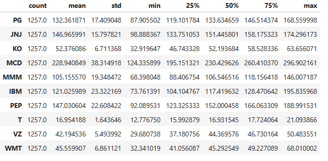
memory usage: 108.0 KB- Checking the descriptive statistics summary
close.describe().T
- Comparing the stock volatility (STD)
close1=close.describe().T
mylabels = ticker_list
y=close1['std']
plt.pie(y, labels = mylabels)
plt.show() 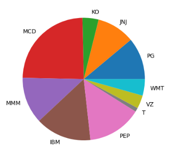
- Calculating and plotting the Market Volume Weights
#Part 2: Creating Weights for Benchmarks
#A. Market Volume Weights
def generateMarketVolumeWeights(close, volume):
    dollar_volume = close * volume
    market_volume_weights = dollar_volume.div(dollar_volume.sum(axis=1), axis=0)

    # Shift the DataFrame by one row
    # As the return for the month depends on the allocation defined in the previous month
    shifted_market_volume_weights = market_volume_weights.shift(1)
    return shifted_market_volume_weights

marketVolumeWeights = generateMarketVolumeWeights(close, volume)
marketVolumeWeights.tail()

PG JNJ KO MCD MMM IBM PEP T VZ WMT
Date
2024-06-14 00:00:00-04:00 0.116738 0.142376 0.086483 0.114468 0.073156 0.085326 0.126974 0.077607 0.070003 0.106869
2024-06-17 00:00:00-04:00 0.113643 0.109370 0.094340 0.131236 0.049957 0.086670 0.108842 0.073683 0.076666 0.155593
2024-06-18 00:00:00-04:00 0.153279 0.131725 0.089292 0.086931 0.047499 0.074344 0.121733 0.065670 0.119059 0.110469
2024-06-20 00:00:00-04:00 0.126916 0.132060 0.098247 0.109189 0.051144 0.085057 0.086290 0.089613 0.101087 0.120398
2024-06-21 00:00:00-04:00 0.161550 0.146852 0.093968 0.116639 0.040140 0.093293 0.093561 0.066024 0.080913 0.107061

marketVolumeWeights.plot(figsize=(12,6))
plt.grid()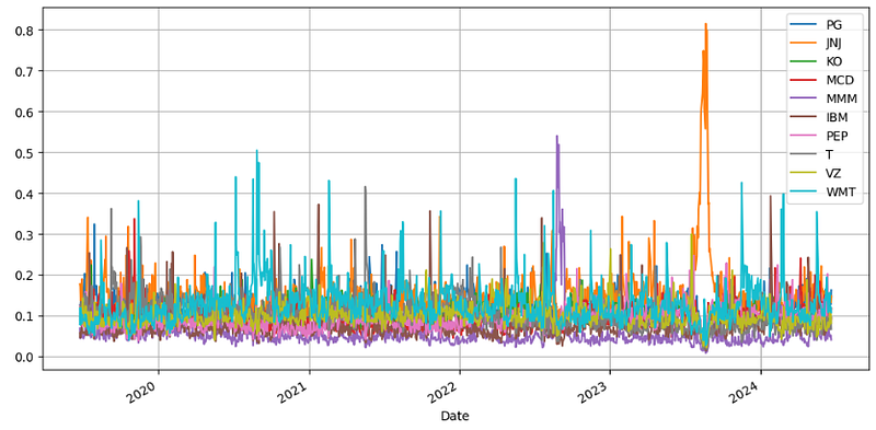
- Calculating and plotting the Dividend Yield Weights
#B. Dividend Yield Weights
def calculateDividendYieldWeights(dividends):
    dividend_cumsum = dividends.cumsum()
    dividend_yield_weights = dividend_cumsum.div(dividend_cumsum.sum(axis=1), axis=0)

    # Shift the DataFrame by one row
    # As the return for the month depends on the allocation defined in the previous month
    shifted_dividend_yield_weights = dividend_yield_weights.shift(1)
    return shifted_dividend_yield_weights

dividendYieldWeights = calculateDividendYieldWeights(dividends)

dividendYieldWeights.plot(figsize=(12,6))
plt.grid()
plt.title('Portfolio 2: Dividend Yield Weights')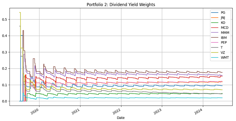
- Generating and plotting the daily returns of Portfolio 2
#C. Returns
def generate_returns(prices):
    return_prices = (prices / prices.shift(1)) - 1
    return return_prices

returns = generate_returns(close)
returns.tail()

PG JNJ KO MCD MMM IBM PEP T VZ WMT
Date
2024-06-14 00:00:00-04:00 0.002283 0.000619 0.000720 -0.000473 -0.006303 0.000532 0.002939 -0.001698 -0.002765 0.004798
2024-06-17 00:00:00-04:00 0.004257 0.002817 0.001119 -0.000276 -0.003667 0.001714 0.014224 0.001701 -0.005294 0.005968
2024-06-18 00:00:00-04:00 0.006328 -0.002056 0.000160 -0.010729 0.002387 0.006195 0.002046 0.021505 0.015712 0.002670
2024-06-20 00:00:00-04:00 -0.005280 0.014624 -0.007185 0.012002 0.008832 0.019760 0.001201 0.003324 0.003992 0.006065
2024-06-21 00:00:00-04:00 0.003519 0.006564 0.009489 0.022025 0.007181 -0.008395 0.003600 0.016013 0.000000 -0.001470

returns.plot(figsize=(12,6))
plt.grid()
plt.title('Daily Returns')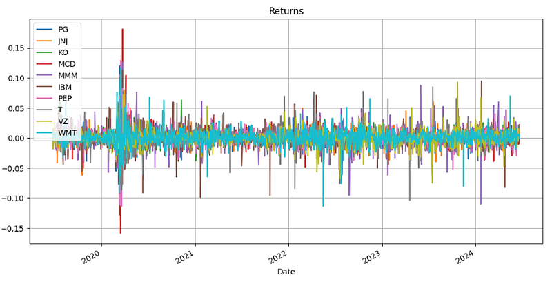
- Generating and plotting the Market Volume Weights Returns
#D. Weighted Returns
def generate_weighted_returns(returns, weights):
    return returns * weights

marketVolumeWeightsReturn = generate_weighted_returns(returns, marketVolumeWeights)
dividendYieldWeightsReturns = generate_weighted_returns(returns, dividendYieldWeights)

marketVolumeWeightsReturn.plot(figsize=(12,6))
plt.grid()
plt.title('Market Volume Weights Returns')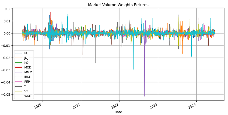
- Plotting the Market Yield Weights Returns
dividendYieldWeightsReturns.plot(figsize=(12,6))
plt.grid()
plt.title('Market Yield Weights Returns')
plt.legend(loc="upper left")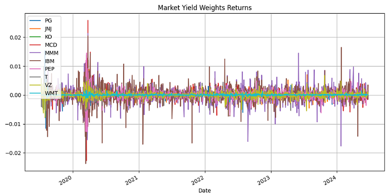
- Calculating and plotting the Cumulative Returns
#E. Cumulative Returns
def calculate_cumulative_returns(returns):
    return (1 + returns.sum(axis = 1)).cumprod()

marketVolumeWeightsCumulativeReturn = calculate_cumulative_returns(marketVolumeWeightsReturn)
dividendYieldWeightsCumulativeReturn = calculate_cumulative_returns(dividendYieldWeightsReturns)

plt.figure(figsize=(10, 4))

plt.plot(marketVolumeWeightsCumulativeReturn, label='Market Volume Portfolio Cumulative Returns', alpha=0.8, color='darkblue')
plt.plot(dividendYieldWeightsCumulativeReturn, label='Dividend Yield Portfolio Cumulative Returns', alpha=0.8, color='royalblue')

plt.title('Cumulative Returns Over Time')
plt.xlabel('Date')
plt.ylabel('Cumulative Returns')
plt.legend(loc='upper left')
plt.grid(True, which='both', linestyle='--', linewidth=0.5)
plt.tight_layout()

plt.show()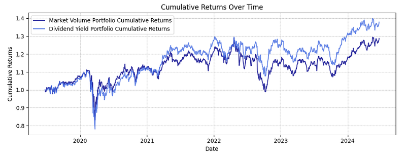
- Implementing Part 3: Portfolio Optimization (Smart Beta Strategy)
#A. Covariance matrix
def get_covariance_returns(returns):
    return np.cov(returns.T.fillna(0))

covariance_returns = get_covariance_returns(returns)
covariance_returns = pd.DataFrame(covariance_returns, returns.columns, returns.columns)

covariance_returns

      PG      JNJ      KO       MCD      MMM      IBM      PEP       T       VZ      WMT
PG 0.000175 0.000099 0.000114 0.000095 0.000092 0.000103 0.000137 0.000098 0.000084 0.000097
JNJ 0.000099 0.000157 0.000092 0.000082 0.000099 0.000100 0.000103 0.000088 0.000070 0.000071
KO 0.000114 0.000092 0.000174 0.000113 0.000114 0.000121 0.000138 0.000115 0.000084 0.000075
MCD 0.000095 0.000082 0.000113 0.000215 0.000115 0.000120 0.000117 0.000099 0.000066 0.000065
MMM 0.000092 0.000099 0.000114 0.000115 0.000310 0.000160 0.000107 0.000126 0.000081 0.000069
IBM 0.000103 0.000100 0.000121 0.000120 0.000160 0.000280 0.000120 0.000142 0.000093 0.000073
PEP 0.000137 0.000103 0.000138 0.000117 0.000107 0.000120 0.000191 0.000109 0.000086 0.000106
T 0.000098 0.000088 0.000115 0.000099 0.000126 0.000142 0.000109 0.000275 0.000149 0.000067
VZ 0.000084 0.000070 0.000084 0.000066 0.000081 0.000093 0.000086 0.000149 0.000170 0.000061
WMT 0.000097 0.000071 0.000075 0.000065 0.000069 0.000073 0.000106 0.000067 0.000061 0.000197

covariance_returns.style.background_gradient(cmap='coolwarm')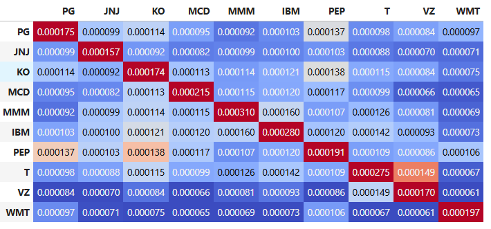
- Importing cvxpy and invoking the weight optimization function
!pip install cvxpy

#B. Weight Optimization
import cvxpy as cvx

def get_optimal_weights(covariance_returns, index_weights, scale=2.0):

    # Create a variable to store the portfolio weights.
    x = cvx.Variable(len(index_weights))

    # Calculate the portfolio variance using the quadratic form.
    portfolio_var = cvx.quad_form(x, covariance_returns)

    # Calculate the distance (L2 norm) between the portfolio weights and the index weights.
    dist_index = cvx.norm(x - index_weights, p=2)

    # Define the objective function: Minimize portfolio variance and distance from the index.
    objective = cvx.Minimize(portfolio_var + scale * dist_index)

    # Define the constraints: Weights should be positive and sum up to 1.
    constraints = [x >= 0, sum(x) == 1]

    # Set up the optimization problem.
    problem = cvx.Problem(objective, constraints)

    # Solve the optimization problem.
    problem.solve()

    # Return the optimal portfolio weights.
return x.value- Rebalancing portfolio over time with chunk_size = 250 (the size of the window over which covariance is calculated) and shift_size = 5 (the number of periods after which the portfolio will be rebalanced)
#C. Rebalance Portfolio Over Time
def rebalance_portfolio(returns, index_weights, shift_size, chunk_size):

    # Initialize an empty list to store the rebalanced portfolio weights at each interval.
    all_rebalance_weights = []

    # List to store the rebalancing dates.
    rebalance_dates = []

    # Iterate through the historical data in steps of shift_size starting from chunk_size.
    for i in range(chunk_size, len(returns), shift_size):

        # Calculate the covariance matrix of returns over the chunk_size window up to the current period.
        covariance_returns = get_covariance_returns(returns.iloc[i-chunk_size:i])

        # Get the optimal portfolio weights using the covariance matrix and the latest index weights.
        rebalance_weights = get_optimal_weights(covariance_returns, index_weights.iloc[i-1])

        # Append the calculated optimal weights to our list.
        all_rebalance_weights.append(rebalance_weights)

        # Append the rebalance date to our dates list.
        rebalance_dates.append(returns.index[i])

    # Convert the list of optimal weights to a DataFrame with columns named after the assets.
    df_rebalance_weights = pd.DataFrame(all_rebalance_weights, columns=returns.columns)

    # Set the rebalance dates as the index of the resulting DataFrame.
    df_rebalance_weights['Date'] = rebalance_dates
    df_rebalance_weights.set_index('Date', inplace=True)

    # Return the DataFrame.
    return df_rebalance_weights

# Define the size of the window over which covariance is calculated.
chunk_size = 250

# Define the number of periods after which the portfolio will be rebalanced.
shift_size = 5

# Rebalance the portfolio
marketVolumeRebalanceWeights = rebalance_portfolio(returns, marketVolumeWeights, shift_size, chunk_size)

# Rebalance the portfolio
dividendYieldRebalanceWeights = rebalance_portfolio(returns, dividendYieldWeights, shift_size, chunk_size)- Plotting the Dividend Yield Rebalance Weights
dividendYieldRebalanceWeights.plot(figsize=(12,6))
plt.grid()
plt.title('Dividend Yield Rebalanced Weights')
plt.legend(loc="upper left")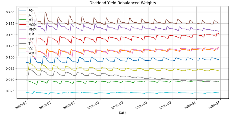
- Plotting the Market Volume Rebalance Weights
marketVolumeRebalanceWeights.plot(figsize=(12,6))
plt.grid()
plt.title('Market Volume Rebalanced Weights')
plt.legend(loc="upper left")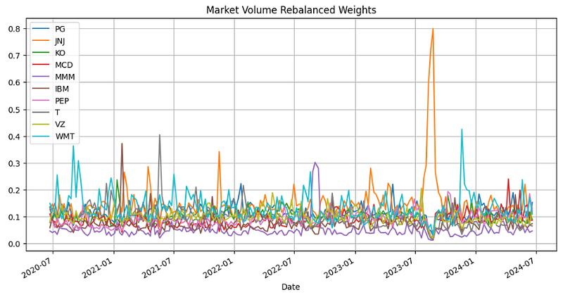
- Calculating the portfolio cumulative returns
#D. Cumulative Returns Calculation
def calculate_cumulative_portfolio_returns(returns, rebalance_weights):
    # Initializing the series for portfolio returns
    portfolio_returns = pd.Series(index=returns.index)

    # Example usage of the function with example data
    n_col = len(rebalance_weights.columns)
    initial_weights = pd.Series([1/n_col] * n_col, index=rebalance_weights.columns)

    # Setting current weights to initial weights
    current_weights = initial_weights

    # Iterating through each date in the returns dataframe
    for date, daily_returns in returns.iterrows():
        if date != returns.index.min():
            # Check if there's a rebalance for this date and update weights if needed
            if date in rebalance_weights.index:
                current_weights = rebalance_weights.loc[date]

            # Calculating the daily portfolio return
            portfolio_return = (daily_returns * current_weights).sum()
            portfolio_returns[date] = portfolio_return

            # Adjusting current_weights based on daily returns
            current_weights *= (1 + daily_returns)

            # Normalizing the weights so they sum up to 1
            current_weights /= current_weights.sum()

    # Calculating cumulative portfolio returns
    cumulative_portfolio_returns = (1 + portfolio_returns).cumprod()

    return cumulative_portfolio_returns

# Calculate cumulative returns
optimizedmarketVolumeWeightsCumulativeReturn = calculate_cumulative_portfolio_returns(returns, marketVolumeRebalanceWeights)
optimizeddividendYieldWeightsCumulativeReturn = calculate_cumulative_portfolio_returns(returns, dividendYieldRebalanceWeights)- Comparing Market Volume Portfolio Cumulative Returns vs Dividend Yield Portfolio Cumulative Returns
fig, (ax1, ax2) = plt.subplots(1, 2, figsize=(12, 4))

ax1.plot(marketVolumeWeightsCumulativeReturn, label='Market Volume Portfolio', alpha=0.8, color='darkblue')
ax1.plot(optimizedmarketVolumeWeightsCumulativeReturn, label='Optimized Market Volume Portfolio', alpha=0.8, color='green')
ax1.set_title('Market Volume Portfolio Cumulative Returns')
ax1.set_xlabel('Date')
ax1.set_ylabel('Cumulative Returns')
ax1.legend(loc='lower right')
ax1.grid(True, which='both', linestyle='--', linewidth=0.5)

ax2.plot(dividendYieldWeightsCumulativeReturn, label='Dividend Yield Portfolio', alpha=0.8, color='royalblue')
ax2.plot(optimizeddividendYieldWeightsCumulativeReturn, label='Optimized Dividend Yield Portfolio', alpha=0.8, color='green')
ax2.set_title('Dividend Yield Portfolio Cumulative Returns')
ax2.set_xlabel('Date')
ax2.set_ylabel('Cumulative Returns')
ax2.legend(loc='lower right')
ax2.grid(True, which='both', linestyle='--', linewidth=0.5)

plt.tight_layout()
plt.show()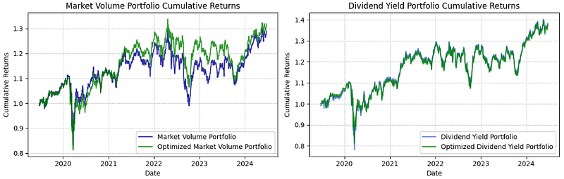
- Comparing the Return/Volatility Ratios before/after PO: Market Volume Portfolio vs Dividend Yield Portfolio
#E. Return to Volatility Ratio
def return_to_volatility_ratio(portfolio_returns):
    mean_return = portfolio_returns.mean()
    std_return = portfolio_returns.std()
    ratio = mean_return / std_return
    return ratio

# Calculating return_to_volatility_ratio for each portfolio
ratios = {
    'Market Volume Portfolio': return_to_volatility_ratio(marketVolumeWeightsCumulativeReturn.diff().dropna()),
    'Optimized Market Volume Portfolio': return_to_volatility_ratio(optimizedmarketVolumeWeightsCumulativeReturn.diff().dropna()),
    'Dividend Yield Portfolio': return_to_volatility_ratio(dividendYieldWeightsCumulativeReturn.diff().dropna()),
    'Optimized Dividend Yield Portfolio': return_to_volatility_ratio(optimizeddividendYieldWeightsCumulativeReturn.diff().dropna())
}

plt.figure(figsize=(10, 6))
plt.bar(ratios.keys(), ratios.values(), color=['darkblue', 'green', 'royalblue', 'green'])
plt.title('Return to Volatility Ratio Comparison')
plt.ylabel('Return to Volatility Ratio')
plt.xticks(rotation=45)
plt.grid(axis='y')
plt.tight_layout()
plt.show()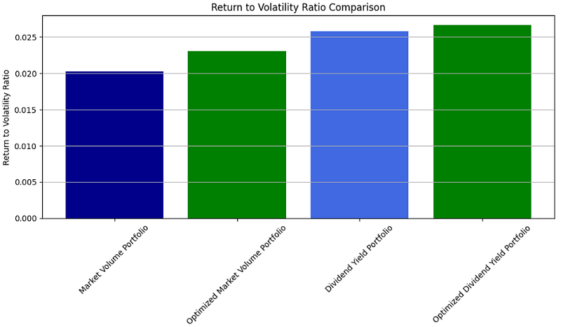
Breakout Strategy Stock Analysis (Portfolio 3)
Here, we’ll discuss the Breakout Strategy with the emphasis on the Shapiro-Wilk (SW) and Kolmogorov-Smirnov (KS) statistical tests in analyzing stock return distributions, viz. Part 1: Fetching Stock Data; Part 2: Compute the Highs and Lows in a Window; Part 3: Compute Long and Short Signals; Part 4: Filter Signal; Part 5: Lookahead Close Prices & Price Returns; Part 6: Compute the Signal Return; Part 7: Analysis and Visualization of Signal Returns.
- Importing the necessary libraries and defining 5Y Portfolio 3 (10 stocks)
# Import necessary libraries
import yfinance as yf
import pandas as pd
from datetime import datetime, timedelta
import numpy as np
import json
import plotly.graph_objects as go
import matplotlib.pyplot as plt

ticker_list = ['AAPL', 'AMZN', 'MSFT', 'GOOGL', 'META', 'TSLA', 'NVDA', 'ADBE', 'NFLX', 'INTC']
years = 5- Part 1: Fetching Stock Data
#Part 1: Fetching Stock Data
def fetch_stock_data(ticker_list, years=5):
    end_date = datetime.now()
    start_date = end_date - timedelta(days=years * 365)

    close_data_df = pd.DataFrame()
    high_data_df = pd.DataFrame()
    low_data_df = pd.DataFrame()

    for ticker in ticker_list:
        stock = yf.Ticker(ticker)

        hist_data = stock.history(period='1d', start=start_date, end=end_date)

        close_data = hist_data['Close'].rename(ticker)
        close_data_df = pd.merge(close_data_df, pd.DataFrame(close_data), left_index=True, right_index=True, how='outer')

        high_data = hist_data['High'].rename(ticker)
        high_data_df = pd.merge(high_data_df, pd.DataFrame(high_data), left_index=True, right_index=True, how='outer')

        low_data = hist_data['Low'].rename(ticker)
        low_data_df = pd.merge(low_data_df, pd.DataFrame(low_data), left_index=True, right_index=True, how='outer')

    return close_data_df, high_data_df, low_data_df

close, high, low = fetch_stock_data(ticker_list, years)- Part 2: Compute the Highs and Lows in a 50-day Window
#Part 2: Compute the Highs and Lows in a Window
def get_high_lows_lookback(high, low, lookback_days):
    lookback_high = high.shift(1).rolling(lookback_days).max()
    lookback_low = low.shift(1).rolling(lookback_days).min()

    return lookback_high, lookback_low

lookback_days = 50
lookback_high, lookback_low = get_high_lows_lookback(high, low, lookback_days)- Part 3: Compute Long and Short Signals
#Part 3: Compute Long and Short Signals
def get_long_short(close, lookback_high, lookback_low):
    long_signal = (close-lookback_high > 0).astype('int')
    short_signal = -(close-lookback_low < 0).astype('int')
    long_short = short_signal + long_signal

    return long_short

signal = get_long_short(close, lookback_high, lookback_low)- Part 4: Filter Signal
#Part 4: Filter Signal
def clear_signals(signals, window_size):
    clean_signals = [0]*window_size

    for signal_i, current_signal in enumerate(signals):
        has_past_signal = bool(sum(clean_signals[signal_i:signal_i+window_size]))
        clean_signals.append(not has_past_signal and current_signal)

    clean_signals = clean_signals[window_size:]

    return pd.Series(np.array(clean_signals).astype(int), signals.index)

def filter_signals(signal, lookahead_days):

    long_signals = (signal > 0 ).astype('int')
    short_signals = -(signal < 0 ).astype('int')

    long_signals = long_signals.apply(lambda s: clear_signals(s, window_size = lookahead_days))
    short_signals = short_signals.apply(lambda s: clear_signals(s, window_size = lookahead_days))

    filtered_signal = long_signals + short_signals

    return filtered_signal

signal_5 = filter_signals(signal, 5)
signal_10 = filter_signals(signal, 10)
signal_20 = filter_signals(signal, 20)- Part 5: Lookahead Close Prices & Price Returns
#Part 5: Lookahead Close Prices & Price Returns
def get_lookahead_prices(close, lookahead_days):
    lookahead_prices = close.shift(-lookahead_days)

    return lookahead_prices

lookahead_5 = get_lookahead_prices(close, 5)
lookahead_10 = get_lookahead_prices(close, 10)
lookahead_20 = get_lookahead_prices(close, 20)

def get_return_lookahead(close, lookahead_prices):
    lookahead_returns = np.log(lookahead_prices/close)

    return lookahead_returns

price_return_5 = get_return_lookahead(close, lookahead_5)
price_return_10 = get_return_lookahead(close, lookahead_10)
price_return_20 = get_return_lookahead(close, lookahead_20)- Part 6: Compute the Signal Return
#Part 6: Compute the Signal Return
def get_signal_return(signal, lookahead_returns):
    signal_return = signal * lookahead_returns

    return signal_return

signal_return_5 = get_signal_return(signal_5, price_return_5)
signal_return_10 = get_signal_return(signal_10, price_return_10)
signal_return_20 = get_signal_return(signal_20, price_return_20)- Plotting Signal 5 Return
import matplotlib.pyplot as plt
signal_return_5.plot(figsize=(14,6))
plt.grid()
plt.title("Signal 5 Return")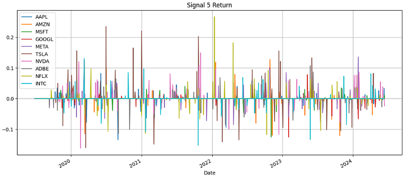
- Plotting Signal 10 Return
signal_return_10.plot(figsize=(14,6))
plt.grid()
plt.legend(loc="lower left")
plt.title("Signal 10 Return")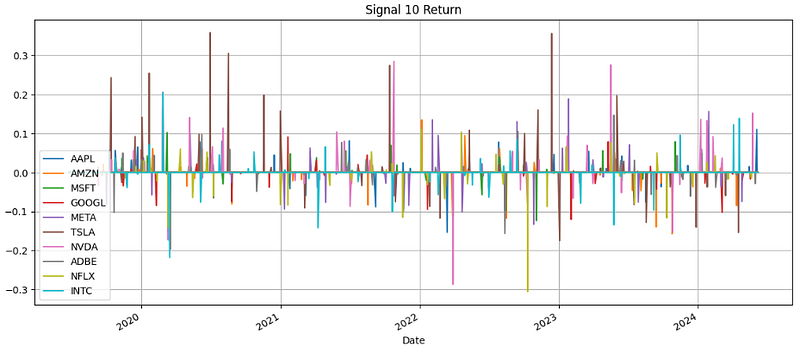
- Plotting Signal 20 Return
signal_return_20.plot(figsize=(14,6))
plt.grid()
plt.legend(loc="lower left")
plt.title("Signal 20 Return")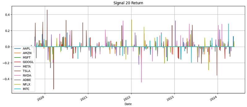
- See Appendix A v.i. for further details of the Breakout Strategy Stock Analysis (Portfolio 3).
Momentum Strategy Stock Analysis (Portfolio 3)
- In this section, we’ll share our experience with implementing a momentum trading strategy that relies on the price moving average, viz. Part 1: Fetching Stock Data; Part 2: Momentum Strategy Simulation; Part 3: Simulating Individual Stock Investments; Part 4: Calculating ROI/Risk Metrics; Part 5: Visualization Summary of Investment Results.
- Our focus will be the market momentum that measures an asset’s speed or velocity — the greater the momentum, the longer a price trend can sustain itself.
- Importing the necessary libraries
# Import necessary libraries
import yfinance as yf
import pandas as pd
from datetime import datetime, timedelta
import numpy as np
import json
import plotly.graph_objects as go- Part 1: Fetching Stock Data
#Part 1: Fetching Stock Data
def fetch_stock_data(ticker_list, years=5):
    end_date = datetime.now()
    start_date = end_date - timedelta(days=years * 365)
    stock_data = pd.DataFrame()

    for ticker in ticker_list:
        stock = yf.Ticker(ticker)
        hist_data = stock.history(period='1d', start=start_date, end=end_date)
        close_data = hist_data['Close'].rename(ticker)
        stock_data = pd.merge(stock_data, pd.DataFrame(close_data), left_index=True, right_index=True, how='outer')
    return stock_data

# Fetch the data
ticker_list = ['AAPL', 'AMZN', 'MSFT', 'GOOGL', 'META', 'TSLA', 'NVDA', 'ADBE', 'NFLX', 'INTC']
years = 5
daily_data = fetch_stock_data(ticker_list, years)

daily_data

                           AAPL     AMZN       MSFT      GOOGL       META       TSLA       NVDA   ADBE       NFLX      INTC
Date
2019-06-26 00:00:00-04:00 48.206604 94.891502 127.728485 53.954075 187.275162 14.618000 3.958648 288.720001 362.200012 42.258209
2019-06-27 00:00:00-04:00 48.192123 95.213997 127.938271 53.769791 189.111389 14.856000 4.057328 293.230011 370.019989 41.618061
2019-06-28 00:00:00-04:00 47.753010 94.681503 127.757080 54.077934 192.604202 14.897333 4.082186 294.649994 367.320007 41.977592
2019-07-01 00:00:00-04:00 48.628838 96.109497 129.397415 54.936951 192.604202 15.144667 4.130407 300.970001 374.600006 42.135429
2019-07-02 00:00:00-04:00 48.913532 96.715500 130.255768 55.566227 194.600113 14.970000 4.032472 301.390015 375.429993 42.196819
... ... ... ... ... ... ... ... ... ... ...
2024-06-14 00:00:00-04:00 212.490005 183.660004 442.570007 176.789993 504.160004 178.009995 131.880005 525.309998 669.380005 30.450001
2024-06-17 00:00:00-04:00 216.669998 184.059998 448.369995 177.240005 506.630005 187.440002 130.979996 518.739990 675.830017 30.980000
2024-06-18 00:00:00-04:00 214.289993 182.809998 446.339996 175.089996 499.489990 184.860001 135.580002 522.250000 685.669983 30.629999
2024-06-20 00:00:00-04:00 209.679993 186.100006 445.700012 176.300003 501.700012 181.570007 130.779999 522.950012 679.030029 30.620001
2024-06-21 00:00:00-04:00 207.490005 189.080002 449.779999 179.630005 494.779999 183.009995 126.570000 533.440002 686.119995 31.090000
1256 rows × 10 columns- Part 2: Momentum Strategy Simulation with initial_amount = 100k
#Part 2: Momentum Strategy Simulation
# Resample data to different frequencies: daily, weekly, monthly
def resample_data(data, period):
    if period == 'D':
        return data
    elif period == 'W':
        return data.resample('W').last()
    elif period == 'M':
        return data.resample('M').last()

# Simulate a simple momentum strategy based on log returns
def simulate_momentum_strategy(data, initial_amount, top_n, tax_rate, period='M'):
    data = resample_data(data, period)
    log_returns = np.log(data / data.shift(1))
    simulation_details = pd.DataFrame(index=log_returns.index,
                                      columns=['Selected Stocks', 'Profit Before Tax', 'Tax Paid', 'Portfolio Value'])
    cash = initial_amount

    # Logic to select top stocks and calculate portfolio value
    for i in range(0, len(log_returns) - 1):
        # Identify the top_n performing stocks based on past log returns
        top_stocks = log_returns.iloc[i].sort_values(ascending=False).head(top_n)
        # Filter out stocks with negative returns
        top_stocks = top_stocks[top_stocks > 0]

        if not top_stocks.empty:
            simulation_details.loc[log_returns.index[i + 1], 'Selected Stocks'] = json.dumps(top_stocks.index.tolist())
            # Calculate the amount to allocate for each stock
            num_stocks = len(top_stocks)
            allocation_per_stock = cash / num_stocks
            # Calculate new portfolio value based on the next day's returns
            new_value = sum(allocation_per_stock * np.exp(log_returns.loc[log_returns.index[i + 1], stock]) for stock in top_stocks.index)
            # Calculate and deduct tax if there is a profit
            profit = new_value - cash
            simulation_details.loc[log_returns.index[i + 1], 'Profit Before Tax'] = round(profit, 2)

            if profit > 0:
                tax = profit * tax_rate
                new_value -= tax
                simulation_details.loc[log_returns.index[i + 1], 'Tax Paid'] = round(tax, 2)
            simulation_details.loc[log_returns.index[i + 1], 'Portfolio Value'] = round(new_value, 2)

        else:
            # No allocation, so portfolio value remains the same
            simulation_details.loc[log_returns.index[i + 1], 'Portfolio Value'] = cash
        # Update cash amount for the next round
        cash = simulation_details.loc[log_returns.index[i + 1], 'Portfolio Value']
    # Assign the initial amount to the first row
    simulation_details.loc[log_returns.index[0], 'Portfolio Value'] = initial_amount
    return simulation_details

# Configuration for the momentum strategy simulation
initial_amount = 100000
top_n = 3
tax_rate = 0.15
frequency = 'M'
simulation_details = simulate_momentum_strategy(daily_data, initial_amount, top_n, tax_rate, frequency)

simulation_details

Selected Stocks Profit Before Tax Tax Paid Portfolio Value
Date
2019-06-30 00:00:00-04:00 NaN NaN NaN 100000
2019-07-31 00:00:00-04:00 NaN NaN NaN 100000
2019-08-31 00:00:00-04:00 ["GOOGL", "TSLA", "AAPL"] -3513.24 NaN 96486.76
2019-09-30 00:00:00-04:00 ["MSFT"] 818.87 122.83 97182.8
2019-10-31 00:00:00-04:00 ["INTC", "AAPL", "TSLA"] 16687.67 2503.15 111367.32
... ... ... ... ...
2024-02-29 00:00:00-05:00 ["NVDA", "NFLX", "META"] 128147.57 19222.14 736860.1
2024-03-31 00:00:00-04:00 ["NVDA", "META", "AMZN"] 37672.64 5650.9 768881.85
2024-04-30 00:00:00-04:00 ["NVDA", "GOOGL", "INTC"] -70586.48 NaN 698295.37
2024-05-31 00:00:00-04:00 ["GOOGL", "TSLA"] 10942.48 1641.37 707596.48
2024-06-30 00:00:00-04:00 ["NVDA", "NFLX", "AAPL"] 71516.88 10727.53 768385.83
61 rows × 4 columns- Part 3: Simulating Individual Stock Investments
#Part 3: Simulating Individual Stock Investments
# Simulate how each individual stock would have performed over the same period
def track_individual_investments(data, initial_amount, simulation_details, period='W'):
    # Resample data based on the specified period
    data = resample_data(data, period)
    # Calculate returns based on the resampled data
    returns = data.pct_change()
    # Create a new DataFrame to store individual stock values over time
    individual_investments = pd.DataFrame(index=data.index, columns=data.columns)
    for stock in data.columns:
        # Simulate an investment in each stock
        individual_investments[stock] = (1 + returns[stock]).cumprod() * initial_amount
    # Include the Portfolio Value from the momentum strategy
    individual_investments['Portfolio Value'] = simulation_details['Portfolio Value']
    individual_investments['Baseline'] = individual_investments.iloc[:, :-1].T.mean()
    # Adjust the first values to match the Initial Amount.
    individual_investments.iloc[0, :] = initial_amount
    return individual_investments.fillna(0).astype(int)

individual_investments_df = track_individual_investments(daily_data, initial_amount, simulation_details, frequency)

individual_investments_df

                          AAPL   AMZN   MSFT   GOOGL  META  TSLA    NVDA ADBE NFLX INTC Portfolio Value Baseline
Date
2019-06-30 00:00:00-04:00 100000 100000 100000 100000 100000 100000 100000 100000 100000 100000 100000 100000
2019-07-31 00:00:00-04:00 107639 98582 101724 112504 100637 108122 102733 101428 87931 105598 100000 102690
2019-08-31 00:00:00-04:00 105867 93803 103254 109949 96202 100962 102098 96558 79971 99707 96486 98837
2019-09-30 00:00:00-04:00 113591 91671 104130 112776 92269 107791 106096 93755 72857 108372 97182 100331
2019-10-31 00:00:00-04:00 126164 93822 107380 116254 99300 140929 122522 94325 78245 118887 111367 109783
... ... ... ... ... ... ... ... ... ... ... ... ...
2024-02-29 00:00:00-05:00 377997 186689 323187 255744 254222 1355141 1937731 190151 164140 102139 736860 514714
2024-03-31 00:00:00-04:00 358611 190512 328719 278777 251862 1180009 2213240 171254 165340 104797 768881 524312
2024-04-30 00:00:00-04:00 356206 184830 304193 300664 223122 1230287 2116388 157077 149907 72292 698295 509497
2024-05-31 00:00:00-04:00 402592 186351 324936 318618 242137 1195381 2685424 150945 174676 73491 707596 575455
2024-06-30 00:00:00-04:00 434506 199701 352058 332168 256889 1228474 3100544 181041 186790 74063 768385 634624
61 rows × 12 columns- Plotting Portfolio Value vs Baseline
plt.figure(figsize=(10, 6))
individual_investments_df['Portfolio Value'].plot(label='Portfolio Value')
individual_investments_df['Baseline'].plot(label='Baseline')
plt.legend()
plt.grid()
plt.title('Portfolio Value vs Baseline')
plt.show()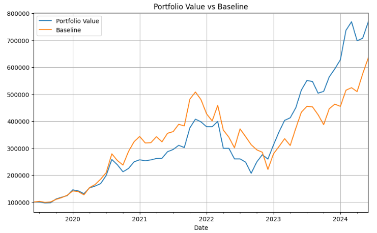
- Plotting Individual Cumulative Returns vs Portfolio Value & Baseline
individual_investments_df.plot(figsize=(12, 6))
plt.title('Individual Cumulative Returns')
plt.grid()
plt.show()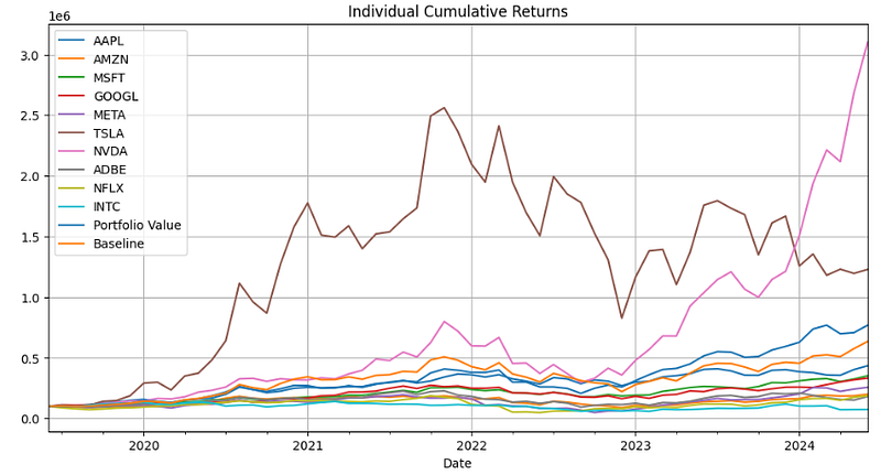
- Part 4: Calculating Metrics
#Part 4: Calculating Metrics
from scipy.stats import ttest_1samp

def calculate_sharpe_ratio(returns, annual_risk_free_rate=0.01, frequency='D'):
    # Adjust the risk-free rate based on the frequency
    if frequency == 'D':
        adjusted_rfr = (1 + annual_risk_free_rate) ** (1/252) - 1
    elif frequency == 'W':
        adjusted_rfr = (1 + annual_risk_free_rate) ** (1/52) - 1
    elif frequency == 'M':
        adjusted_rfr = (1 + annual_risk_free_rate) ** (1/12) - 1

    excess_returns = returns - adjusted_rfr
    return excess_returns.mean() / excess_returns.std()

def t_test_portfolio_returns(portfolio_returns, bench_annual_rate=0.1, frequency='D'):
    # Adjust the risk-free rate based on the frequency
    if frequency == 'D':
        adjusted_rfr = (1 + bench_annual_rate) ** (1/252) - 1
    elif frequency == 'W':
        adjusted_rfr = (1 + bench_annual_rate) ** (1/52) - 1
    elif frequency == 'M':
        adjusted_rfr = (1 + bench_annual_rate) ** (1/12) - 1

    t_stat, p_value = ttest_1samp(portfolio_returns[1:], adjusted_rfr)  # [1:] to exclude the NaN from pct_change
    return t_stat, p_value

def calculate_metrics(dataframe, initial_amount, bench_annual_rate, frequency='D'):
    # Calculate the final and relative values
    final_values = dataframe.iloc[-1]
    relative_values = final_values / initial_amount - 1  # Subtract 1 to get the growth proportion

    # Calculate mean return and Sharpe Ratio
    returns = dataframe.pct_change()

    if frequency == 'D':
        annualization_factor = 252
    elif frequency == 'W':
        annualization_factor = 52
    elif frequency == 'M':
        annualization_factor = 12

    # Corrected annualization of mean returns
    mean_returns = (1 + returns.mean()) ** annualization_factor - 1
    sharpes = returns.apply(calculate_sharpe_ratio, annual_risk_free_rate=0.01, frequency=frequency)

    # Test if the portfolio returns are greater than the adjusted risk-free rate
    portfolio_returns = dataframe['Portfolio Value'].pct_change()
    t_stat, p_value = t_test_portfolio_returns(portfolio_returns, bench_annual_rate, frequency=frequency)

    return final_values, relative_values, mean_returns, sharpes, t_stat, p_value / 2

bench_annual_rate = 0.1

# Calculate the metrics
final_values, relative_values, mean_returns, sharpes, t_stat, p_value = calculate_metrics(individual_investments_df, initial_amount, bench_annual_rate, frequency)- Plotting the Sharpe Ratios
sharpes.plot.bar(figsize=(12, 6))
plt.title('Sharpe Ratios')
plt.grid()
plt.show()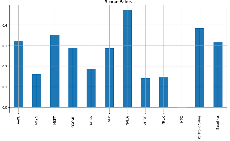
- Printing the p-value and t-statistic
print(p_value)
0.009201411022319347

print(t_stat)
2.424687499520688

mean_returns.plot.bar(figsize=(12, 6))
plt.title('Mean Returns')
plt.grid()
plt.show()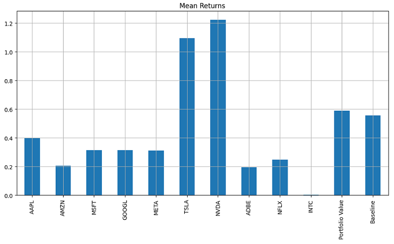
- Plotting Relative Values
relative_values.plot.bar(figsize=(12, 6))
plt.title('Relative Values')
plt.grid()
plt.show()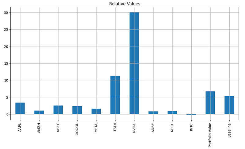
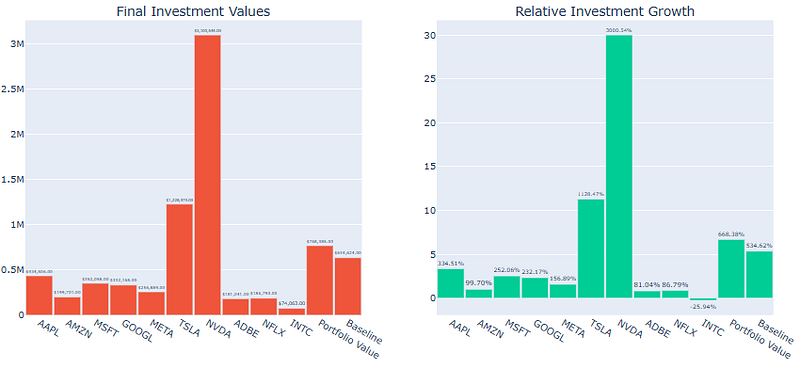
- Plotting Final Values
final_values.plot.bar(figsize=(12, 6))
plt.title('Final Values')
plt.grid()
plt.show()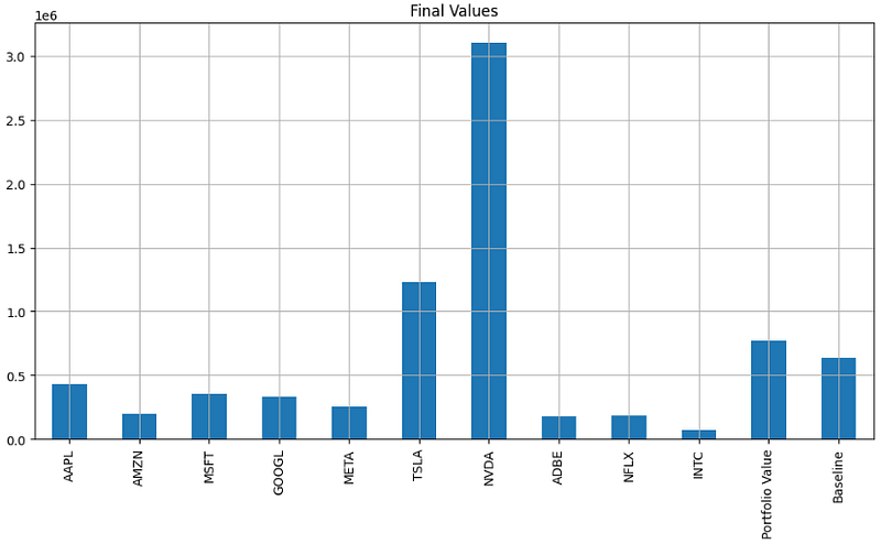
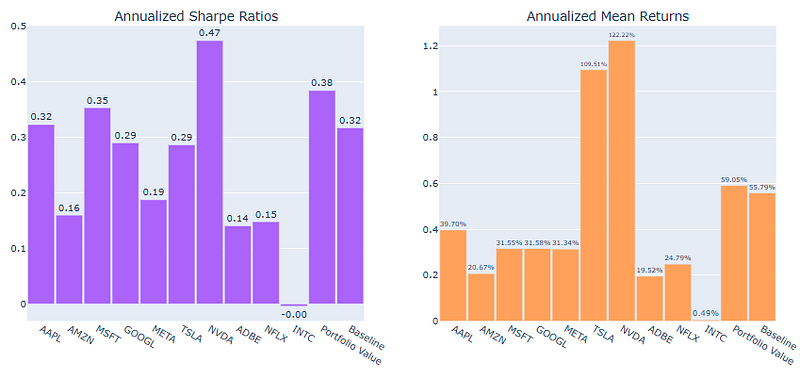
- Part 5: Final Visualization
#Part 5: Visualization
import plotly.graph_objects as go
from plotly.subplots import make_subplots

def plot_combined_charts(dataframe, final_values, relative_values, sharpes, mean_returns):
    labels = final_values.index
    colors = ['#636EFA', '#EF553B', '#00CC96', '#AB63FA', '#FFA15A']

    fig = make_subplots(rows=3, cols=2,
                        subplot_titles=('Portfolio Value Over Time',
                                        '',
                                        'Final Investment Values',
                                        'Relative Investment Growth',
                                        'Annualized Sharpe Ratios',
                                        'Annualized Mean Returns'),
                        vertical_spacing=0.08)

    # Portfolio Value line chart
    fig.add_trace(go.Scatter(x=dataframe.index,
                             y=dataframe['Portfolio Value'],
                             mode='lines',
                             name='Portfolio Value',
                             line=dict(color=colors[0], width=2.5)),
                  row=1, col=1)

    # T-test and P-value
    significance_text = f"T-test: {t_stat:.2f}P-value: {p_value:.5f}"
    if t_stat > 2 and p_value < 0.05:
        significance_text += f"Significantly different from {bench_annual_rate:.0%} per year!"

    fig.add_annotation(
        text=significance_text,
        showarrow=False,
        xref="x2", yref="y2",
        x=0.5, y=0.5,
        font=dict(size=15),
        bgcolor="white",
        align="center"
    )

    # Final values
    fig.add_trace(go.Bar(x=labels,
                         y=final_values.values,
                         name='Final Values ($)',
                         text=[f"${v:,.2f}" for v in final_values.values],
                         textposition='outside',
                         marker_color=colors[1]),
                  row=2, col=1)

    # Relative Growth
    fig.add_trace(go.Bar(x=labels,
                         y=relative_values.values,
                         name='Relative Growth',
                         text=[f"{v:.2%}" for v in relative_values.values],
                         textposition='outside',
                         marker_color=colors[2]),
                  row=2, col=2)

    # Sharpe Ratios
    fig.add_trace(go.Bar(x=labels,
                         y=sharpes.values,
                         name='Annualized Sharpe Ratio',
                         text=[f"{v:.2f}" for v in sharpes.values],
                         textposition='outside',
                         marker_color=colors[3]),
                  row=3, col=1)

    # Mean Returns
    fig.add_trace(go.Bar(x=labels,
                         y=mean_returns.values,
                         name='Annualized Mean Returns',
                         text=[f"{v:.2%}" for v in mean_returns.values],
                         textposition='outside',
                         marker_color=colors[4]),
                  row=3, col=2)

    # Update layout
    fig.update_layout(title_text="Investment Results Overview",
                      title_font=dict(size=24, color='black', family="Arial Black"),
                      title_pad=dict(t=10),
                      showlegend=False,
                      height=1500,
                      title_x=0.5,
                      bargap=0.05,
                      )

    fig.show()

plot_combined_charts(individual_investments_df, final_values, relative_values, sharpes, mean_returns)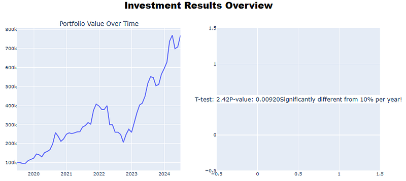
Using Stock Fundamentals (Portfolio 4)
- Some momentum strategies emphasize fundamental analysis factors, such as quarterly or annual earnings per share (EPS) and other metrics, to avoid making emotional decisions.
- In this section, we will explain in detail how to retrieve stock data and financial statements using yfinance [13, 14] and relevant data visualizations [14].
- For simplicity, let’s consider only 2 big tech stocks, such as MSFT and NVDA (Portfolio 4).
- Importing libraries
import pandas as pd
import yahoo_fin.stock_info as si
import yfinance as yf

import plotly.express as px
import plotly.graph_objects as go
import matplotlib.pyplot as plt


%matplotlib inline- MSFT 5Y Candlesticks, Price Charts vs Volume
company = 'MSFT'   # Ticker of the company to be analyzed
df = yf.Ticker(company).history(period='5y',interval='1d')
fig = go.Figure(data=[go.Candlestick(x=df.index,
                open=df['Open'],
                high=df['High'],
                low=df['Low'],
                close=df['Close'])])

fig.update_layout(title = f'{company}: Candlestick Price Chart', xaxis_tickfont_size = 14)
fig.update_layout(xaxis_rangeslider_visible = False)

fig.show()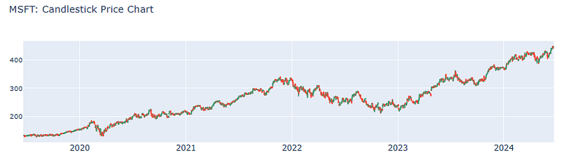
plt.style.use('ggplot')
top = plt.subplot2grid((4,4), (0, 0), rowspan=3, colspan=4)
top.plot(df.index, df["Close"], color='blue')
plt.title(f'{company}: Price Chart')

bottom = plt.subplot2grid((4,4), (3,0), rowspan=1, colspan=4)
bottom.bar(df.index, df['Volume'], color='black')
plt.title('Volume')
plt.gcf().set_size_inches(17,8)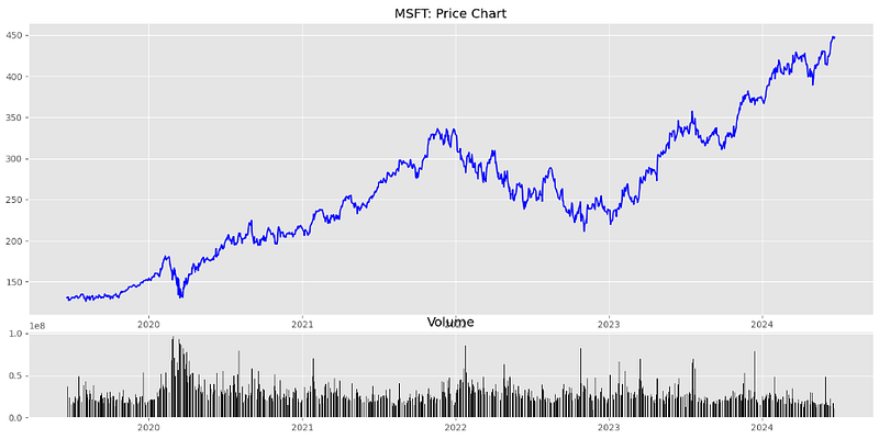
- Examining the MSFT Total Revenues USD for the available time period
# Import yfinance
import yfinance as yf

# Set the ticker as MSFT
msft = yf.Ticker("MSFT")

# show revenues
plt.figure(figsize=(13,6))
revenue = msft.financials.loc['Total Revenue']
plt.bar(revenue.index, revenue.values,width = 100)
plt.ylabel("MSFT Total Revenues USD")
plt.xlabel("Date")
plt.show()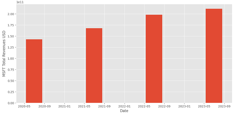
- Plotting the NVDA Total Revenues USD for the available time period
nvda = yf.Ticker("NVDA")
plt.figure(figsize=(13,6))
revenue = nvda.financials.loc['Total Revenue']
plt.bar(revenue.index, revenue.values,width = 100)
plt.ylabel("NVDA Total Revenues USD")
plt.xlabel("Date")
plt.grid()
plt.show()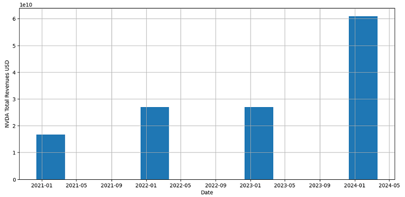
- Printing and plotting the NVDA balance sheet
nvda.balance_sheet
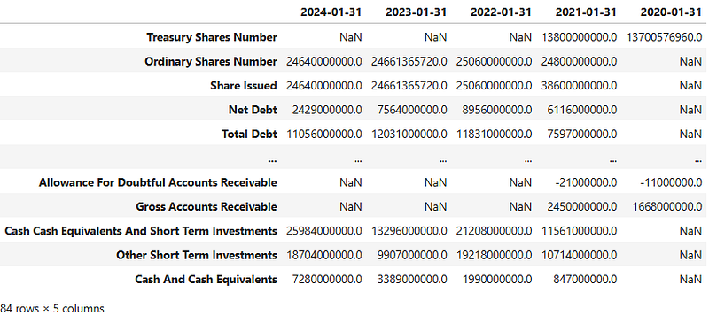
bs=nvda.balance_sheet
bs['2024-01-31'].plot.bar(figsize=(20,5))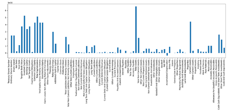
- Plotting the NVDA cashflow on 2024–01–31
cf=nvda.cashflow
cf['2024-01-31'].plot.bar(figsize=(20,5))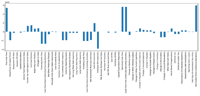
- Fetch the full company info
nvda.info

# cf. Appendix B

ninfo=nvda.info
ninfo['revenueGrowth']
2.621
The Altman Z-Score Revisited (Portfolio 5)
- Based on the above fundamental analysis , we’ll calculate the Altman Z-Score [12] by adopting the relevant Python functions and importing the required libraries such as
- yfinance: to access financial market data; imported as yf
- pandas : DataFrame and other utilities; imported as pd
- numpy: for nan; imported as np
- The Altman Z-Score assesses a company’s financial health and likelihood of bankruptcy based on multiple fundamental financial metrics to be discussed below.
- We’ll consider 5Y Portfolio 5:
ticker_list = ['MSFT','AAPL','AMZN','META','INTC','AMD','GEN']- Working with the MSFT balance sheet
msft.balance_sheet
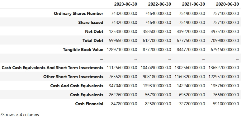
- Example fetching the MSFT Cash Financial on 2023–06–30
msbs=msft.balance_sheet
msbs1=msbs['2023-06-30']
msbs1['Cash Financial']
8478000000.0- Calculating ratio_x_1: working capital / total assets [12]
msbs1['Current Assets']
184257000000.0

working_capital = msbs1['Current Assets'] - msbs1['Current Liabilities']
total_assets = msbs1['Total Assets']
ratio_x_1=working_capital/total_assets

print(ratio_x_1)
0.1944482202846768- Calculating all 5 fundamental ratios [12]
import yfinance as yf

msft = yf.Ticker("MSFT")

ticker="MSFT"
date='2023-06-30'

# ratio_x_1: working capital / total assets
def ratio_x_1(ticker,date) -> float:
    msft=yf.Ticker(ticker)
    msbs=msft.balance_sheet
    df=msbs[date]
    working_capital = df['Current Assets'] - df['Current Liabilities']
    total_assets = df['Total Assets']
    return working_capital/total_assets

ratio_1=ratio_x_1(ticker,date)
print(ratio_1)
0.1944482202846768

def ratio_x_2(ticker,date) -> float:
    msft=yf.Ticker(ticker)
    msbs=msft.balance_sheet
    df=msbs[date]
    retained_earnings = df['Retained Earnings']
    total_assets = df['Total Assets']
    return retained_earnings/total_assets

ratio_2=ratio_x_2(ticker,date)
print(ratio_2)
0.28848282424218885

# earnings before interest and tax / total assets
def ratio_x_3(ticker,date) -> float:
    msft=yf.Ticker(ticker)
    msbs=msft.income_stmt
    df = msbs[date]
    ebit = df['EBIT']

    msbs1=msft.balance_sheet
    df1=msbs1[date]
    total_assets = df1['Total Assets']

    return ebit/total_assets

ratio_3=ratio_x_3(ticker,date)
print(ratio_3)
0.22156387750742762


# market value of equity / total liabilities
def ratio_x_4(ticker,date) -> float:
    msft=yf.Ticker(ticker)
    msin=msft.info
    equity_market_value = msin['sharesOutstanding'] * msin['currentPrice']
    msbs=msft.balance_sheet
    df=msbs[date]
    total_liabilities = df['Total Liabilities Net Minority Interest']
    return equity_market_value/total_liabilities

ratio_4=ratio_x_4(ticker,date)
print(ratio_4)
16.247171530197857

# sales / total assets
def ratio_x_5(ticker,date) -> float:
    msft=yf.Ticker(ticker)
    msbs=msft.income_stmt
    df = msbs[date]
    sales = df['Total Revenue']
    msbs1=msft.balance_sheet
    df1=msbs1[date]
    total_assets = df1['Total Assets']
    return sales/total_assets

ratio_5=ratio_x_5(ticker,date)
print(ratio_5)
0.5143867603938094
- Calculating the MSFT Z-score by summing the above 5 ratios
def z_score(ticker,date) -> float:
    ratio_1 = ratio_x_1(ticker,date)
    ratio_2 = ratio_x_2(ticker,date)
    ratio_3 = ratio_x_3(ticker,date)
    ratio_4 = ratio_x_4(ticker,date)
    ratio_5 = ratio_x_5(ticker,date)
    # Z = 1.2X1 + 1.4X2 + 3.3X3 + 0.6X4 + 1.0X5.
    zscore = 1.2*ratio_1 + 1.4*ratio_2 + 3.3*ratio_3 + 0.6*ratio_4 + 1.0*ratio_5
    return zscore

msfz=z_score(ticker,date)
print(msfz)

11.631064292567713- Comparing the following 2 tech stocks
ticker_list = ['MSFT','AAPL']
date_list=['2023-06-30','2023-09-30']

symbol_to_score = {}
for i in range(len(ticker_list)):
    ticker=ticker_list[i]
    date=date_list[i]
    zsc=z_score(ticker,date)
    symbol_to_score[ticker]=zsc
    print (i,ticker,date,zsc)

0 MSFT 2023-06-30 11.631064292567713
1 AAPL 2023-09-30 8.754487491097787

print(symbol_to_score)
{'MSFT': 11.631064292567713, 'AAPL': 8.754487491097787}

tmp = yf.Ticker("AAPL")
tmp.balance_sheet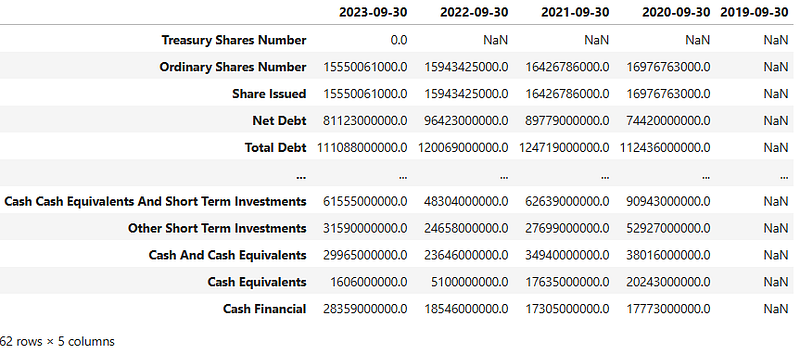
- Introducing the Distress, Grey, and Safe Zones [12]
def highlight_distress(val):
    return 'background-color: indianred' if val != '' else ""

def highlight_grey(val):
    return 'background-color: grey' if val != '' else ""

def highlight_safe(val):
    return 'background-color: green' if val != '' else ""

def format_score(val):
    try:
        return '{:.2f}'.format(float(val))
    except:
        return ''

def make_pretty(styler):
    #1 No index
    styler.hide(axis='index')

    #2 Column formatting
    styler.format(format_score, subset=['Distress Zone', 'Grey Zone', 'Safe Zone'])

    #3 Left text alignment for some columns
    styler.set_properties(subset=['Symbol', 'Distress Zone', 'Grey Zone', 'Safe Zone'], **{'text-align': 'center', 'width': '100px'})

    #4 Apply highlight methods to columns
    styler.map(highlight_grey, subset=['Grey Zone'])
    styler.map(highlight_safe, subset=['Safe Zone'])
    styler.map(highlight_distress, subset=['Distress Zone'])
    return styler

#1 Categorise
SYMBOLS=ticker_list
distress = [''] * len(SYMBOLS)
grey = [''] * len(SYMBOLS)
safe = [''] * len(SYMBOLS)

for idx, zscore in enumerate(symbol_to_score.values()):
    if zscore <= 1.8:
        distress[idx] = zscore
    elif zscore > 1.8 and zscore <= 2.99:
        grey[idx] = zscore
    else:
        safe[idx] = zscore

#2 Create a dictionary for the DF
data_dict = {'Symbol': SYMBOLS, 'Distress Zone': distress, 'Grey Zone': grey, 'Safe Zone': safe}
df = pd.DataFrame.from_dict(data_dict)
#3 Drop any rows with NaN values
df.dropna(inplace=True)

styles = [
    dict(selector='td', props=[('font-size', '10pt'),('border-style','solid'),('border-width','1px')]),
    dict(selector='th.col_heading', props=[('font-size', '11pt'),('text-align', 'center')]),
    dict(selector='caption', props=[('text-align', 'center'),
                                     ('font-size', '14pt'), ('font-weight', 'bold')])
]
#4 Apply styles
df_styled = df.style.set_table_styles(styles)
df.style.pipe(make_pretty).set_caption('Altman Z Score').set_table_styles(styles)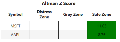
- Printing the full set of balance sheets within Portfolio 5
tmp = yf.Ticker("NVDA")
tmp.balance_sheet
2024-01-31 2023-01-31 2022-01-31 2021-01-31 2020-01-31

tmp = yf.Ticker("AMZN")
tmp.balance_sheet
2023-12-31 2022-12-31 2021-12-31 2020-12-31 2019-12-31

tmp = yf.Ticker("META")
tmp.balance_sheet
2023-12-31 2022-12-31 2021-12-31 2020-12-31 2019-12-31

tmp = yf.Ticker("INTC")
tmp.balance_sheet
2023-12-31 2022-12-31 2021-12-31 2020-12-31 2019-12-31

tmp = yf.Ticker("AMD")
tmp.balance_sheet
2023-12-31 2022-12-31 2021-12-31 2020-12-31 2019-12-31

tmp = yf.Ticker("GEN")
tmp.balance_sheet
2024-03-31 2023-03-31 2022-03-31 2021-03-31 2020-03-31- Calculating the Z-score of the above stocks for the latest available dates
ticker_list = ['MSFT','AAPL','AMZN','META','INTC','AMD','GEN']
date_list=['2023-06-30','2023-09-30','2023-12-31','2023-12-31','2023-12-31','2023-12-31','2024-03-31']
symbol_to_score = {}
for i in range(len(ticker_list)):
    ticker=ticker_list[i]
    date=date_list[i]
    zsc=z_score(ticker,date)
    symbol_to_score[ticker]=zsc
    print (i,ticker,date,zsc)

0 MSFT 2023-06-30 11.631064292567713
1 AAPL 2023-09-30 8.754487491097787
2 AMZN 2023-12-31 5.2835715222038955
3 META 2023-12-31 10.564184819996882
4 INTC 2023-12-31 1.8850700500184252
5 AMD 2023-12-31 13.593729096733899
6 GEN 2024-03-31 1.0462068969351226

#1 Categorise
SYMBOLS=ticker_list
distress = [''] * len(SYMBOLS)
grey = [''] * len(SYMBOLS)
safe = [''] * len(SYMBOLS)

for idx, zscore in enumerate(symbol_to_score.values()):
    if zscore <= 1.8:
        distress[idx] = zscore
    elif zscore > 1.8 and zscore <= 2.99:
        grey[idx] = zscore
    else:
        safe[idx] = zscore

#2 Create a dictionary for the DF
data_dict = {'Symbol': SYMBOLS, 'Distress Zone': distress, 'Grey Zone': grey, 'Safe Zone': safe}
df = pd.DataFrame.from_dict(data_dict)
#3 Drop any rows with NaN values
df.dropna(inplace=True)

styles = [
    dict(selector='td', props=[('font-size', '10pt'),('border-style','solid'),('border-width','1px')]),
    dict(selector='th.col_heading', props=[('font-size', '11pt'),('text-align', 'center')]),
    dict(selector='caption', props=[('text-align', 'center'),
                                     ('font-size', '14pt'), ('font-weight', 'bold')])
]
#4 Apply styles
df_styled = df.style.set_table_styles(styles)
df.style.pipe(make_pretty).set_caption('Altman Z Score').set_table_styles(styles)
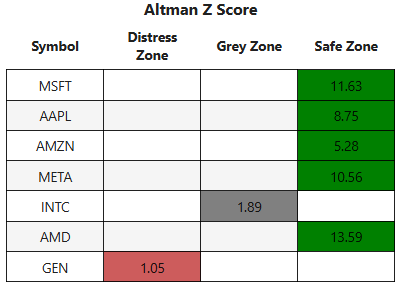
Appendix A: Breakout Strategy Stock Analysis (Continued).
- Plotting Signal Returns 5 vs 10
plt.figure(figsize=(10, 6))
plt.scatter(signal_return_5,signal_return_10)
plt.grid()
plt.xlabel("Signal Return 5")
plt.ylabel("Signal Return 10")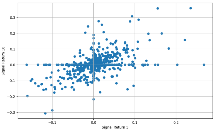
- Plotting Signal Returns 5 vs 20
plt.figure(figsize=(10, 6))
plt.scatter(signal_return_5,signal_return_20)
plt.grid()
plt.xlabel("Signal Return 5")
plt.ylabel("Signal Return 20")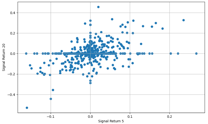
- Plotting Signal Returns 10 vs 20
plt.figure(figsize=(10, 6))
plt.scatter(signal_return_10,signal_return_20)
plt.grid()
plt.xlabel("Signal Return 10")
plt.ylabel("Signal Return 20")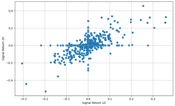
- Part 7: Analysis and Visualization of Signal Returns
from scipy.stats import shapiro, kstest
import matplotlib.pyplot as plt
import warnings

dataframes = [signal_return_5, signal_return_10, signal_return_20]
colors = ['blue', 'green', 'red']
labels = ['signal_return_5', 'signal_return_10', 'signal_return_20']- Plotting histograms of Signal Returns
#A. Plotting histograms of Signal Returns
plt.figure(figsize=(10, 6))

for df, color, label in zip(dataframes, colors, labels):
    # Filter out NaN and zero values and flatten the data
    filtered_data = df.values[~pd.isna(df.values)]
    filtered_data = filtered_data[filtered_data != 0.0]

    # Plot the histogram
    plt.hist(filtered_data, bins=30, edgecolor='black', alpha=0.5, color=color, label=label)

plt.title('Histogram of Signal Returns')
plt.xlabel('Value')
plt.ylabel('Frequency')
plt.legend()
plt.grid()
plt.show()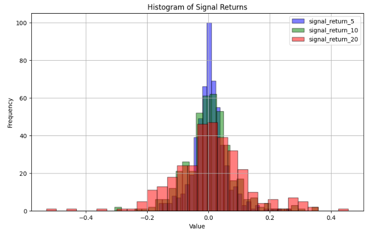
- Test for Normality using the Shapiro-Wilk Test (SWT)
#B. Test for Normality using the Shapiro-Wilk Test
means = []

for df, label in zip(dataframes, labels):
    # Filter out NaN and zero values and flatten the data
    filtered_data = df.values[~pd.isna(df.values)]
    filtered_data = filtered_data[filtered_data != 0.0]

    # Calculate the mean
    mean_val = filtered_data.mean()
    means.append(mean_val)

    # Shapiro-Wilk Test
    stat, p = shapiro(filtered_data)
    alpha = 0.05
    if p > alpha:
        print(f"{label}: Looks Gaussian (fail to reject H0). p-value = {p:.5f}")
    else:
        print(f"{label}: Does not look Gaussian (reject H0). p-value = {p:.5f}")

print("\nMeans of the distributions:")
for label, mean in zip(labels, means):
    print(f"{label}: {mean:.5f}")

signal_return_5: Does not look Gaussian (reject H0). p-value = 0.00000
signal_return_10: Does not look Gaussian (reject H0). p-value = 0.00000
signal_return_20: Does not look Gaussian (reject H0). p-value = 0.00001

Means of the distributions:
signal_return_5: 0.00370
signal_return_10: 0.00467
signal_return_20: 0.00685- Plotting means of the above distributions
mylabels = labels
y=means
myexplode = [0., 0.1, 0.2]
plt.pie(y, labels = mylabels,explode=myexplode)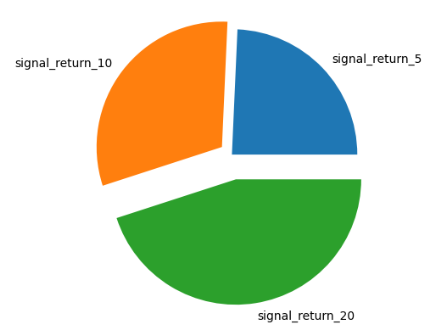
- Comparing the Signal Returns to a Normal Distribution
#C. Comparing the Signal Returns to a Normal Distribution
for df, color, label in zip(dataframes, colors, labels):
    # Filter out NaN and zero values and flatten the data
    filtered_data = df.values[~pd.isna(df.values)]
    filtered_data = filtered_data[filtered_data != 0.0]

    # Parameters for normal distribution
    mean_val = filtered_data.mean()
    std_dev = filtered_data.std()

    # Generate random samples from a normal distribution with the same mean and std_dev
    normal_samples = np.random.normal(mean_val, std_dev, size=len(filtered_data))

    # Plot histograms
    plt.figure(figsize=(6, 5))
    plt.hist(filtered_data, bins=30, edgecolor='black', alpha=0.5, color=color, label=label, density=True)
    plt.hist(normal_samples, bins=30, edgecolor='black', alpha=0.5, color='grey', label='Normal Dist.', density=True, histtype='step')
    plt.title(f'Histogram of {label} vs. Normal Distribution')
    plt.xlabel('Value')
    plt.ylabel('Density')
    plt.legend()
    plt.grid()
    plt.show()
    print('\n')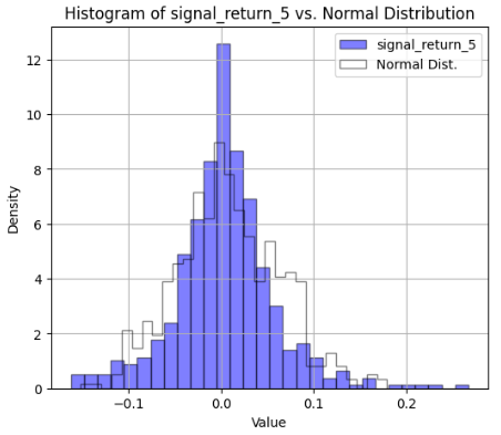
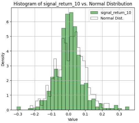
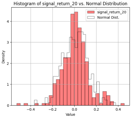
- Kolmogorov-Smirnov (KS) Test to assess the goodness of fit
#D. Kolmogorov-Smirnov Test to assess the goodness of fit
# Filter out returns that don't have a long or short signal.
long_short_signal_returns_5 = signal_return_5[signal_5 != 0].stack()
long_short_signal_returns_10 = signal_return_10[signal_10 != 0].stack()
long_short_signal_returns_20 = signal_return_20[signal_20 != 0].stack()

# Get just ticker and signal return
long_short_signal_returns_5 = long_short_signal_returns_5.reset_index().iloc[:, [1,2]]
long_short_signal_returns_5.columns = ['ticker', 'signal_return']
long_short_signal_returns_10 = long_short_signal_returns_10.reset_index().iloc[:, [1,2]]
long_short_signal_returns_10.columns = ['ticker', 'signal_return']
long_short_signal_returns_20 = long_short_signal_returns_20.reset_index().iloc[:, [1,2]]
long_short_signal_returns_20.columns = ['ticker', 'signal_return']

import pandas as pd
import warnings
from scipy.stats import kstest

warnings.simplefilter(action='ignore', category=FutureWarning)

def calculate_kstest(long_short_signal_returns):
    ks_values = pd.Series(dtype='float64')
    p_values = pd.Series(dtype='float64')

    for ticker, signals in long_short_signal_returns.groupby('ticker')['signal_return']:
        mean = signals.mean()
        std = signals.std(ddof=0)
        standardized_signals = (signals - mean) / std
        ks_value, p_value = kstest(standardized_signals, 'norm')
        ks_values[ticker] = ks_value
        p_values[ticker] = p_value

    return ks_values, p_values

# Calculate KS test values for all three dataframes
ks_values_5, p_values_5 = calculate_kstest(long_short_signal_returns_5)
ks_values_10, p_values_10 = calculate_kstest(long_short_signal_returns_10)
ks_values_20, p_values_20 = calculate_kstest(long_short_signal_returns_20)

# Compile results into a DataFrame
results = pd.DataFrame({
    'ticker': ks_values_5.index,
    'ks_value_5': ks_values_5.values,
    'p_value_5': p_values_5.values,
    'ks_value_10': ks_values_10.values,
    'p_value_10': p_values_10.values,
    'ks_value_20': ks_values_20.values,
    'p_value_20': p_values_20.values,
})

# Use style.bar to display the bars for easier visual comparison
results.style.bar(subset=['ks_value_5', 'p_value_5', 'ks_value_10', 'p_value_10', 'ks_value_20', 'p_value_20'], align='zero', color=['#d65f5f', '#000000'])

ticker ks_value_5 p_value_5 ks_value_10 p_value_10 ks_value_20 p_value_20
0 AAPL 0.111881 0.362906 0.136818 0.313318 0.093808 0.889502
1 ADBE 0.067559 0.941434 0.076082 0.939221 0.069446 0.992809
2 AMZN 0.095484 0.748976 0.089770 0.908827 0.125178 0.670293
3 GOOGL 0.163585 0.104526 0.077354 0.950986 0.139123 0.520547
4 INTC 0.077184 0.916189 0.071082 0.983394 0.146238 0.539062
5 META 0.069942 0.915596 0.089626 0.831141 0.100795 0.846063
6 MSFT 0.131177 0.224118 0.140942 0.316079 0.108387 0.793751
7 NFLX 0.122626 0.419100 0.138855 0.373414 0.107050 0.832704
8 NVDA 0.074000 0.855231 0.102112 0.661011 0.068943 0.993406
9 TSLA 0.066733 0.953433 0.140872 0.400624 0.105686 0.843578- Plotting the above result of the KS Test
results.style.background_gradient(cmap='coolwarm')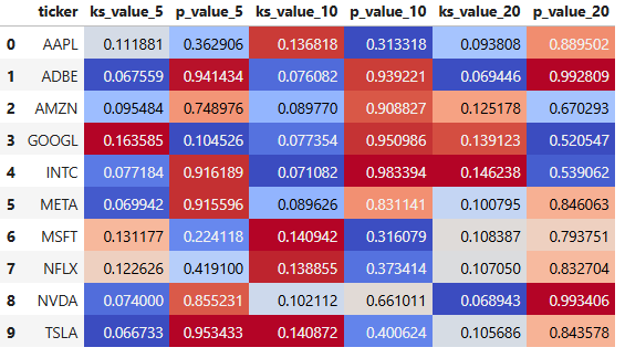
Appendix B: NVDA — Full Company Info
{'address1': '2788 San Tomas Expressway',
 'city': 'Santa Clara',
 'state': 'CA',
 'zip': '95051',
 'country': 'United States',
 'phone': '408 486 2000',
 'website': 'https://www.nvidia.com',
 'industry': 'Semiconductors',
 'industryKey': 'semiconductors',
 'industryDisp': 'Semiconductors',
 'sector': 'Technology',
 'sectorKey': 'technology',
 'sectorDisp': 'Technology',
 'longBusinessSummary': "NVIDIA Corporation provides graphics and compute and networking solutions in the United States, Taiwan, China, Hong Kong, and internationally. The Graphics segment offers GeForce GPUs for gaming and PCs, the GeForce NOW game streaming service and related infrastructure, and solutions for gaming platforms; Quadro/NVIDIA RTX GPUs for enterprise workstation graphics; virtual GPU or vGPU software for cloud-based visual and virtual computing; automotive platforms for infotainment systems; and Omniverse software for building and operating metaverse and 3D internet applications. The Compute & Networking segment comprises Data Center computing platforms and end-to-end networking platforms, including Quantum for InfiniBand and Spectrum for Ethernet; NVIDIA DRIVE automated-driving platform and automotive development agreements; Jetson robotics and other embedded platforms; NVIDIA AI Enterprise and other software; and DGX Cloud software and services. The company's products are used in gaming, professional visualization, data center, and automotive markets. It sells its products to original equipment manufacturers, original device manufacturers, system integrators and distributors, independent software vendors, cloud service providers, consumer internet companies, add-in board manufacturers, distributors, automotive manufacturers and tier-1 automotive suppliers, and other ecosystem participants. NVIDIA Corporation was incorporated in 1993 and is headquartered in Santa Clara, California.",
 'fullTimeEmployees': 29600,
 'companyOfficers': [{'maxAge': 1,
   'name': 'Mr. Jen-Hsun  Huang',
   'age': 60,
   'title': 'Co-Founder, CEO, President & Director',
   'yearBorn': 1963,
   'fiscalYear': 2024,
   'totalPay': 7491487,
   'exercisedValue': 217327152,
   'unexercisedValue': 0},
  {'maxAge': 1,
   'name': 'Ms. Colette M. Kress',
   'age': 56,
   'title': 'Executive VP & CFO',
   'yearBorn': 1967,
   'fiscalYear': 2024,
   'totalPay': 1510765,
   'exercisedValue': 0,
   'unexercisedValue': 0},
  {'maxAge': 1,
   'name': 'Ms. Debora  Shoquist',
   'age': 68,
   'title': 'Executive Vice President of Operations',
   'yearBorn': 1955,
   'fiscalYear': 2024,
   'totalPay': 1371266,
   'exercisedValue': 0,
   'unexercisedValue': 0},
  {'maxAge': 1,
   'name': 'Mr. Timothy S. Teter',
   'age': 56,
   'title': 'Executive VP, General Counsel & Secretary',
   'yearBorn': 1967,
   'fiscalYear': 2024,
   'totalPay': 1360939,
   'exercisedValue': 0,
   'unexercisedValue': 0},
  {'maxAge': 1,
   'name': 'Mr. Ajay K. Puri',
   'age': 68,
   'title': 'Executive Vice President of Worldwide Field Operations',
   'yearBorn': 1955,
   'fiscalYear': 2024,
   'totalPay': 2295097,
   'exercisedValue': 0,
   'unexercisedValue': 0},
  {'maxAge': 1,
   'name': 'Mr. Chris A. Malachowsky',
   'title': 'Co-Founder',
   'fiscalYear': 2024,
   'totalPay': 320000,
   'exercisedValue': 0,
   'unexercisedValue': 0},
  {'maxAge': 1,
   'name': 'Mr. Donald F. Robertson Jr.',
   'age': 54,
   'title': 'VP & Chief Accounting Officer',
   'yearBorn': 1969,
   'fiscalYear': 2024,
   'exercisedValue': 0,
   'unexercisedValue': 0},
  {'maxAge': 1,
   'name': 'Prof. William J. Dally Ph.D.',
   'age': 62,
   'title': 'Chief Scientist & Senior VP of Research',
   'yearBorn': 1961,
   'fiscalYear': 2024,
   'exercisedValue': 0,
   'unexercisedValue': 0},
  {'maxAge': 1,
   'name': 'Ms. Simona  Jankowski C.F.A., J.D.',
   'title': 'Vice President of Investor Relations',
   'fiscalYear': 2024,
   'exercisedValue': 0,
   'unexercisedValue': 0},
  {'maxAge': 1,
   'name': 'Mr. Robert  Sherbin',
   'age': 64,
   'title': 'Vice President of Corporate Communications',
   'yearBorn': 1959,
   'fiscalYear': 2024,
   'exercisedValue': 0,
   'unexercisedValue': 0}],
 'auditRisk': 7,
 'boardRisk': 10,
 'compensationRisk': 1,
 'shareHolderRightsRisk': 6,
 'overallRisk': 7,
 'governanceEpochDate': 1717200000,
 'compensationAsOfEpochDate': 1735603200,
 'irWebsite': 'http://phx.corporate-ir.net/phoenix.zhtml?c=116466&p=irol-IRHome',
 'maxAge': 86400,
 'priceHint': 2,
 'previousClose': 130.78,
 'open': 127.0,
 'dayLow': 124.3,
 'dayHigh': 130.63,
 'regularMarketPreviousClose': 130.78,
 'regularMarketOpen': 127.0,
 'regularMarketDayLow': 124.3,
 'regularMarketDayHigh': 130.63,
 'dividendRate': 0.04,
 'dividendYield': 0.00029999999,
 'exDividendDate': 1718064000,
 'payoutRatio': 0.0094,
 'fiveYearAvgDividendYield': 0.12,
 'beta': 1.694,
 'trailingPE': 74.01754,
 'forwardPE': 35.060944,
 'volume': 600706148,
 'regularMarketVolume': 600706148,
 'averageVolume': 442141975,
 'averageVolume10days': 356877350,
 'averageDailyVolume10Day': 356877350,
 'bid': 126.42,
 'ask': 126.9,
 'bidSize': 100,
 'askSize': 200,
 'marketCap': 3113406955520,
 'fiftyTwoWeekLow': 39.23,
 'fiftyTwoWeekHigh': 140.76,
 'priceToSalesTrailing12Months': 39.02784,
 'fiftyDayAverage': 100.9835,
 'twoHundredDayAverage': 69.40835,
 'trailingAnnualDividendRate': 0.016,
 'trailingAnnualDividendYield': 0.00012234287,
 'currency': 'USD',
 'enterpriseValue': 3093421096960,
 'profitMargins': 0.53398,
 'floatShares': 23599764000,
 'sharesOutstanding': 24598300672,
 'sharesShort': 278905720,
 'sharesShortPriorMonth': 290753620,
 'sharesShortPreviousMonthDate': 1713139200,
 'dateShortInterest': 1715731200,
 'sharesPercentSharesOut': 0.0113,
 'heldPercentInsiders': 0.043169998,
 'heldPercentInstitutions': 0.67643,
 'shortRatio': 0.64,
 'shortPercentOfFloat': 0.0117999995,
 'impliedSharesOutstanding': 25507000320,
 'bookValue': 1.998,
 'priceToBook': 63.348347,
 'lastFiscalYearEnd': 1706400000,
 'nextFiscalYearEnd': 1738022400,
 'mostRecentQuarter': 1714262400,
 'earningsQuarterlyGrowth': 6.284,
 'netIncomeToCommon': 42597998592,
 'trailingEps': 1.71,
 'forwardEps': 3.61,
 'pegRatio': 1.04,
 'lastSplitFactor': '10:1',
 'lastSplitDate': 1717977600,
 'enterpriseToRevenue': 38.777,
 'enterpriseToEbitda': 62.779,
 '52WeekChange': 2.1150324,
 'SandP52WeekChange': 0.26238096,
 'lastDividendValue': 0.01,
 'lastDividendDate': 1718064000,
 'exchange': 'NMS',
 'quoteType': 'EQUITY',
 'symbol': 'NVDA',
 'underlyingSymbol': 'NVDA',
 'shortName': 'NVIDIA Corporation',
 'longName': 'NVIDIA Corporation',
 'firstTradeDateEpochUtc': 917015400,
 'timeZoneFullName': 'America/New_York',
 'timeZoneShortName': 'EDT',
 'uuid': '7f5f6a07-b148-30f4-98a2-2caa3df2aed0',
 'messageBoardId': 'finmb_32307',
 'gmtOffSetMilliseconds': -14400000,
 'currentPrice': 126.57,
 'targetHighPrice': 200.0,
 'targetLowPrice': 47.84,
 'targetMeanPrice': 125.1,
 'targetMedianPrice': 126.75,
 'recommendationMean': 1.8,
 'recommendationKey': 'buy',
 'numberOfAnalystOpinions': 48,
 'totalCash': 31438000128,
 'totalCashPerShare': 1.278,
 'ebitda': 49274998784,
 'totalDebt': 11237000192,
 'quickRatio': 2.877,
 'currentRatio': 3.529,
 'totalRevenue': 79773999104,
 'debtToEquity': 22.866,
 'revenuePerShare': 3.234,
 'returnOnAssets': 0.49103,
 'returnOnEquity': 1.15658,
 'freeCashflow': 29023750144,
 'operatingCashflow': 40524001280,
 'earningsGrowth': 6.5,
 'revenueGrowth': 2.621,
 'grossMargins': 0.75286,
 'ebitdaMargins': 0.61768,
 'operatingMargins': 0.64925003,
 'financialCurrency': 'USD',
 'trailingPegRatio': 1.4499}
Discussion
- Data science plays a crucial role in optimizing the SAA process. This helps in mitigating risks while maximizing returns on investments.
- By leveraging the proposed PO techniques, quants can better understand market trends, identify patterns, and make more accurate predictions.
- The key concepts in data-driven SAA are stock data preprocessing, feature engineering, model selection, and evaluation.
- The proposed technical analysis methods combine well with fundamental analysis to provide additional information to investors.
- By harnessing the power of data science, portfolio managers can gain a significant edge in the marketplace: developing better models for evaluating asset profits and risk factors; automating the execution of trades and PO based on model predictions.
Conclusions
- We have demonstrated how data science can be used in extracting crucial insights from financial market.
- We have presented several SAA/PO use-case examples of optimizing portfolios, backtesting effective trading strategies, and performing detailed stock analysis.
- We have shown how to combine technical and fundamental analysis. Traders often compare the differences between fundamental and technical analysis, however blending the two can have positive benefits.
- We have gained a relatively comprehensive understanding of the application of statistics to investment portfolios. It focuses on the principle of the factor model. We have compared pros and cons of different factors in different situations.
- Generally, the use of data science in portfolio management can provide numerous benefits to asset managers:
- It can improve the PO process by providing more accurate estimates of returns and risk.
- It can also help portfolio managers to better understand the underlying dynamics of the current market conditions, identify opportunities, and make decisions in real-time or close to real-time.
- It is also capable of predicting market movements, enabling portfolio managers to adjust their strategies appropriately.
The Road Ahead
- Exploiting investor sentiment for portfolio optimization.
- Understanding ESG metrics within the concept of 3D investing.
- Insights into Wealth Management in terms of estate planning and tax minimization.
Explore More
- A Market-Neutral Strategy
- Blue-Chip Stock Portfolios for Quant Traders
- Multiple-Criteria Technical Analysis of Blue Chips in Python
- Joint Analysis of Bitcoin, Gold and Crude Oil Prices
- Dividend-NG-BTC Diversify Big Tech
- Applying a Risk-Aware Portfolio Rebalancing Strategy to ETF, Energy, Pharma, and Aerospace/Defense Stocks in 2023
- Towards Max(ROI/Risk) Trading
- Portfolio Optimization of 20 Dividend Growth Stocks
- Stock Portfolio Risk/Return Optimization
- Risk/Return QC via Portfolio Optimization — Current Positions of The Dividend Breeder
- Portfolio Optimization Risk/Return QC — Positions of Humble Div vs Dividend Glenn
- Algorithmic Testing Stock Portfolios to Optimize the Risk/Reward Ratio
References
- A Deep Dive into Risk Modeling for Stock Market Analysis
- Optimizing Investment Portfolios through Smart Beta Strategy
- Stock Analysis with a Breakout Strategy
- Creating and Evaluating Alpha Factors
- Data Science for Financial Markets
- Portfolio Optimization Strategies | Maximize Returns
- Alpha Research and Factor Modeling
- Portfolio optimization using Python
- Portfolio Management
- Quant Investment — how I construct FACTORS for alpha research (feature engineering)
- Quantitative Finance using Python-2: Basic Statistical Methods Using Python for Analyzing Stock
- How to calculate Altman Z-Score using yfinance Python API
- How to Obtain Financial Statements from Stocks Using yfinance
- Stock Market Data: Obtaining Data, Visualization & Analysis in Python
Acknowledgements
Contacts
Disclaimer
- The following disclaimer clarifies that the information provided in this article is for educational use only and should not be considered financial or investment advice.
- The information provided does not take into account your individual financial situation, objectives, or risk tolerance.
- Any investment decisions or actions you undertake are solely your responsibility.
- You should independently evaluate the suitability of any investment based on your financial objectives, risk tolerance, and investment timeframe.
- It is recommended to seek advice from a certified financial professional who can provide personalized guidance tailored to your specific needs.
- The tools, data, content, and information offered are impersonal and not customized to meet the investment needs of any individual. As such, the tools, data, content, and information are provided solely for informational and educational purposes only.


