
Stock Analysis with a Breakout Strategy
In this article, we not only introduce the core of the Breakout Strategy but also emphasize the significance of the Shapiro-Wilk and Kolmogorov-Smirnov tests in analyzing stock return distributions.

Introduction
In a sequel to our initial exploration, which centered on the Momentum-Based Strategy, this paper’s primary focus transitions to the intricacies of the Breakout Strategy. At its core, this strategy revolves around discerning price barriers. Once breached, these barriers often signify the inception of a potentially robust trend in price movement. Such trends, more often than not, originate from points of price resistance or supports, offering traders a unique opportunity to tap into nascent trends, frequently ahead of their peak.
Differentiating itself from the momentum-based strategy, the Breakout Strategy is inherently anticipatory. Instead of capitalizing on ongoing market trends, its objective is to pinpoint moments that foreshadow impending trends through pivotal price shifts. Our evaluation of this strategy won’t just rely on a singular approach; we’ll harness a multifaceted toolkit, one that stresses the importance of understanding stock return distributions. Tools like histogram plotting will be vital, but the essence of our investigation rests on two sophisticated tests: the Shapiro-Wilk Test and the Kolmogorov-Smirnov Test. While the former is renowned for its sensitivity in discerning normal distributions, the latter offers versatility against any distribution type. Both tests will be instrumental in probing the nuances of signal returns, gauging their normality, and confirming their fit in the larger picture.
Our endeavor, therefore, is not just to elucidate the mechanics of the Breakout Strategy, but also to underscore the significance of a meticulous, data-centric approach in deciphering stock markets. We aim to provide traders with a holistic insight into the dynamics of this strategy and its ramifications in today’s fluid market landscape.
Fetching Stock Data
Every analysis begins with data. Using Python’s yfinance package, the past five years of stock data for ten companies - including giants like Apple (AAPL), Amazon (AMZN), Microsoft (MSFT), etc. - were fetched. For each stock, closing prices, high and low prices were extracted.
def fetch_stock_data(ticker_list, years=5):
    end_date = datetime.now()
    start_date = end_date - timedelta(days=years * 365)

    close_data_df = pd.DataFrame()
    high_data_df = pd.DataFrame()
    low_data_df = pd.DataFrame()

    for ticker in ticker_list:
        stock = yf.Ticker(ticker)

        hist_data = stock.history(period='1d', start=start_date, end=end_date)

        close_data = hist_data['Close'].rename(ticker)
        close_data_df = pd.merge(close_data_df, pd.DataFrame(close_data), left_index=True, right_index=True, how='outer')

        high_data = hist_data['High'].rename(ticker)
        high_data_df = pd.merge(high_data_df, pd.DataFrame(high_data), left_index=True, right_index=True, how='outer')

        low_data = hist_data['Low'].rename(ticker)
        low_data_df = pd.merge(low_data_df, pd.DataFrame(low_data), left_index=True, right_index=True, how='outer')

    return close_data_df, high_data_df, low_data_df

# Fetch the data
ticker_list = ['AAPL', 'AMZN', 'MSFT', 'GOOGL', 'META', 'TSLA', 'NVDA', 'ADBE', 'NFLX', 'INTC']
years = 5

close, high, low = fetch_stock_data(ticker_list, years)
Computing the Highs and Lows in a Window
For a momentum-based strategy, one crucial step is determining the highs and lows for a stock within a given window of time. For this analysis, a window of 50 days was considered. The rolling maximum and minimum prices for each stock within this window were computed.
def get_high_lows_lookback(high, low, lookback_days):
    lookback_high = high.shift(1).rolling(lookback_days).max()
    lookback_low = low.shift(1).rolling(lookback_days).min()

    return lookback_high, lookback_low

lookback_days = 50
lookback_high, lookback_low = get_high_lows_lookback(high, low, lookback_days)
Generating Long and Short Signals
The core of a momentum-based strategy is determining when to buy (or go long) and when to sell (or go short) based on price movements. A simple logic was used: if the current closing price is greater than the high of the past 50 days, a long signal is triggered. Conversely, if it’s less than the low of the past 50 days, a short signal is issued.
def get_long_short(close, lookback_high, lookback_low):
    long_signal = (close-lookback_high > 0).astype('int')
    short_signal = -(close-lookback_low < 0).astype('int')
    long_short = short_signal + long_signal

    return long_short

signal = get_long_short(close, lookback_high, lookback_low)
Filtering the Signals
When dealing with trading signals, overlapping indications within a short timeframe can lead to excessive trading. To mitigate this, we employ two functions:
clear_signalsfilters out new signals within a givenwindow_sizeif a previous signal exists.filter_signalsdifferentiates between buy (long_signals) and sell (short_signals) indications, applies the clear function, and then consolidates them.
By doing this, the signals are simplified, allowing us to focus more on the distinct and potentially more effective trading signals.
def clear_signals(signals, window_size):
    clean_signals = [0]*window_size

    for signal_i, current_signal in enumerate(signals):
        has_past_signal = bool(sum(clean_signals[signal_i:signal_i+window_size]))
        clean_signals.append(not has_past_signal and current_signal)

    clean_signals = clean_signals[window_size:]

    return pd.Series(np.array(clean_signals).astype(int), signals.index)

def filter_signals(signal, lookahead_days):

    long_signals = (signal > 0 ).astype('int')
    short_signals = -(signal < 0 ).astype('int')

    long_signals = long_signals.apply(lambda s: clear_signals(s, window_size = lookahead_days))
    short_signals = short_signals.apply(lambda s: clear_signals(s, window_size = lookahead_days))

    filtered_signal = long_signals + short_signals

    return filtered_signal

signal_5 = filter_signals(signal, 5)
signal_10 = filter_signals(signal, 10)
signal_20 = filter_signals(signal, 20)
Anticipating Future Prices and Analyzing Price Returns
Future prices were anticipated using a simple shift mechanism. This lookahead helps in understanding possible returns. Returns, calculated using the logarithmic difference between the lookahead prices and the current prices, are crucial for determining the profitability of a trading strategy.
Note: In this analysis, trading operation costs have not been taken into account.
def get_lookahead_prices(close, lookahead_days):
    lookahead_prices = close.shift(-lookahead_days)

    return lookahead_prices

lookahead_5 = get_lookahead_prices(close, 5)
lookahead_10 = get_lookahead_prices(close, 10)
lookahead_20 = get_lookahead_prices(close, 20)
def get_return_lookahead(close, lookahead_prices):
lookahead_returns = np.log(lookahead_prices/close)
return lookahead_returns
price_return_5 = get_return_lookahead(close, lookahead_5)
price_return_10 = get_return_lookahead(close, lookahead_10)
price_return_20 = get_return_lookahead(close, lookahead_20)Deriving the Signal Return
By multiplying the signal with the lookahead returns, the expected return for each stock based on our strategy was computed. This effectively means what one would earn (or lose) if they followed the signals.
def get_signal_return(signal, lookahead_returns):
    signal_return = signal * lookahead_returns

    return signal_return

signal_return_5 = get_signal_return(signal_5, price_return_5)
signal_return_10 = get_signal_return(signal_10, price_return_10)
signal_return_20 = get_signal_return(signal_20, price_return_20)
Analyzing and Visualizing the Signal Returns
Here, we will scrutinize the returns generated from our trading signals, emphasizing their distribution and statistical properties. Through a mix of visualizations and statistical tests, we aim to understand the nature of these returns and pinpoint any anomalies or outliers.
Histograms of Signal Returns
Histograms provide a visual representation of the distribution of a dataset. The histograms for returns over 5, 10, and 20 days were plotted. Interestingly, all signal returns exhibited deviations from a standard normal distribution.
from scipy.stats import shapiro, kstest
import matplotlib.pyplot as plt
import warnings

dataframes = [signal_return_5, signal_return_10, signal_return_20]
colors = ['blue', 'green', 'red']
labels = ['signal_return_5', 'signal_return_10', 'signal_return_20']plt.figure(figsize=(10, 6))
for df, color, label in zip(dataframes, colors, labels):
# Filter out NaN and zero values and flatten the data
filtered_data = df.values[~pd.isna(df.values)]
filtered_data = filtered_data[filtered_data != 0.0]
# Plot the histogram
plt.hist(filtered_data, bins=30, edgecolor='black', alpha=0.5, color=color, label=label)
plt.title('Histogram of Signal Returns')
plt.xlabel('Value')
plt.ylabel('Frequency')
plt.legend()
plt.show()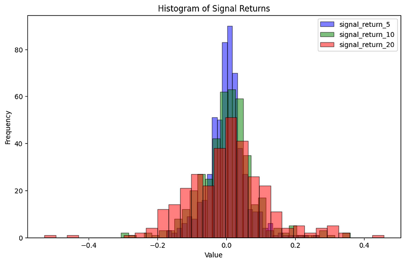
Testing for Normality
The assumption of normality is fundamental in many statistical methods. Thus, evaluating whether the distribution of returns resembles a Gaussian distribution is crucial.
We used the Shapiro-Wilk Test, a prevalent method for normality testing. The hypothesis (H0) for this test is that the data was drawn from a normal distribution. The p-value indicates the strength of the evidence against this hypothesis. Generally, a lower p-value would mean that we reject H0, suggesting the data is not normally distributed.
means = []

for df, label in zip(dataframes, labels):
    # Filter out NaN and zero values and flatten the data
    filtered_data = df.values[~pd.isna(df.values)]
    filtered_data = filtered_data[filtered_data != 0.0]

    # Calculate the mean
    mean_val = filtered_data.mean()
    means.append(mean_val)

    # Shapiro-Wilk Test
    stat, p = shapiro(filtered_data)
    alpha = 0.05
    if p > alpha:
        print(f"{label}: Looks Gaussian (fail to reject H0). p-value = {p:.5f}")
    else:
        print(f"{label}: Does not look Gaussian (reject H0). p-value = {p:.5f}")

print("\nMeans of the distributions:")
for label, mean in zip(labels, means):
    print(f"{label}: {mean:.5f}")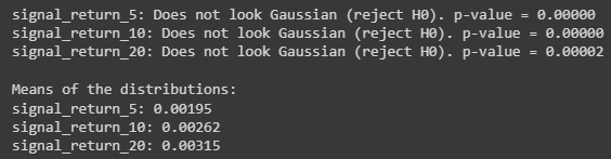
From our analysis:
- signal_return_5 has a p-value of approximately zero, thus does not follow a Gaussian distribution.
- signal_return_10 exhibits a similar trend with a p-value of approximately zero.
- signal_return_20 is consistent with the previous two with a p-value of 0.00002 (very low).
Given these minuscule p-values, we confidently reject the hypothesis that our returns are drawn from a normal distribution for all three signal durations.
Furthermore, the means of the distributions provide insight into the average returns:
- Average return for signal_return_5 is 0.00195.
- Average return for signal_return_10 is 0.00262.
- Average return for signal_return_20 is 0.00315.
It’s evident that the means of the distributions increment with longer signal durations. However, it’s essential to balance this against the potential increase in risk associated with such returns.
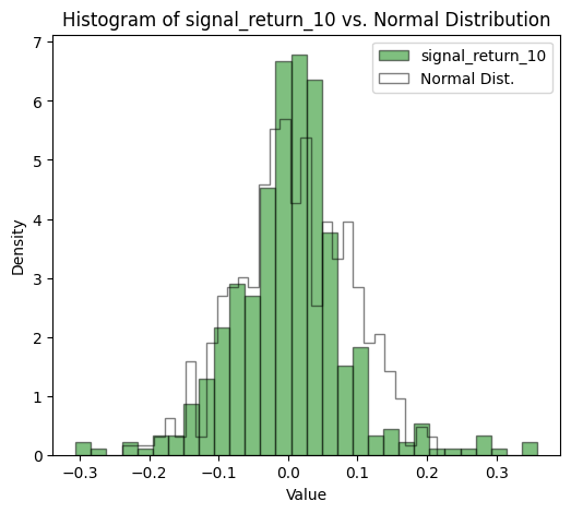
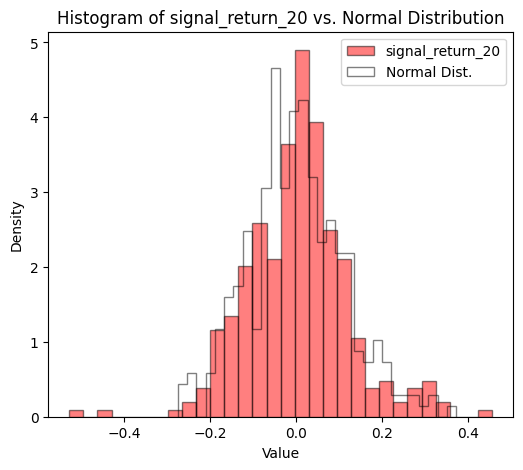
Comparing Signal Returns to a Normal Distribution
While the data didn’t seem to follow a normal distribution, the significance of this observation was emphasized when comparing the signal returns with an actual normal distribution. The discrepancies were evident.
for df, color, label in zip(dataframes, colors, labels):
    # Filter out NaN and zero values and flatten the data
    filtered_data = df.values[~pd.isna(df.values)]
    filtered_data = filtered_data[filtered_data != 0.0]

    # Parameters for normal distribution
    mean_val = filtered_data.mean()
    std_dev = filtered_data.std()

    # Generate random samples from a normal distribution with the same mean and std_dev
    normal_samples = np.random.normal(mean_val, std_dev, size=len(filtered_data))

    # Plot histograms
    plt.figure(figsize=(6, 5))
    plt.hist(filtered_data, bins=30, edgecolor='black', alpha=0.5, color=color, label=label, density=True)
    plt.hist(normal_samples, bins=30, edgecolor='black', alpha=0.5, color='grey', label='Normal Dist.', density=True, histtype='step')
    plt.title(f'Histogram of {label} vs. Normal Distribution')
    plt.xlabel('Value')
    plt.ylabel('Density')
    plt.legend()
    plt.show()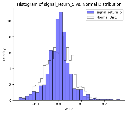
Goodness of Fit
In our analysis, we utilized the Kolmogorov-Smirnov (KS) test to assess the alignment of returns for various stocks with a normal distribution. This approach was carefully chosen to compare individual stock returns with a normal distribution defined by the mean and standard deviation of the aggregated stock returns.
# Filter out returns that don't have a long or short signal.
long_short_signal_returns_5 = signal_return_5[signal_5 != 0].stack()
long_short_signal_returns_10 = signal_return_10[signal_10 != 0].stack()
long_short_signal_returns_20 = signal_return_20[signal_20 != 0].stack()

# Get just ticker and signal return
long_short_signal_returns_5 = long_short_signal_returns_5.reset_index().iloc[:, [1,2]]
long_short_signal_returns_5.columns = ['ticker', 'signal_return']
long_short_signal_returns_10 = long_short_signal_returns_10.reset_index().iloc[:, [1,2]]
long_short_signal_returns_10.columns = ['ticker', 'signal_return']
long_short_signal_returns_20 = long_short_signal_returns_20.reset_index().iloc[:, [1,2]]
long_short_signal_returns_20.columns = ['ticker', 'signal_return']
import pandas as pd
import warnings
from scipy.stats import kstest
warnings.simplefilter(action='ignore', category=FutureWarning)
def calculate_kstest(long_short_signal_returns):
ks_values = pd.Series(dtype='float64')
p_values = pd.Series(dtype='float64')
for ticker, signals in long_short_signal_returns.groupby('ticker')['signal_return']:
mean = signals.mean()
std = signals.std(ddof=0)
standardized_signals = (signals - mean) / std
ks_value, p_value = kstest(standardized_signals, 'norm')
ks_values[ticker] = ks_value
p_values[ticker] = p_value
return ks_values, p_values
# Calculate KS test values for all three dataframes
ks_values_5, p_values_5 = calculate_kstest(long_short_signal_returns_5)
ks_values_10, p_values_10 = calculate_kstest(long_short_signal_returns_10)
ks_values_20, p_values_20 = calculate_kstest(long_short_signal_returns_20)
# Compile results into a DataFrame
results = pd.DataFrame({
'ticker': ks_values_5.index,
'ks_value_5': ks_values_5.values,
'p_value_5': p_values_5.values,
'ks_value_10': ks_values_10.values,
'p_value_10': p_values_10.values,
'ks_value_20': ks_values_20.values,
'p_value_20': p_values_20.values,
})
# Use style.bar to display the bars for easier visual comparison
results.style.bar(subset=['ks_value_5', 'p_value_5', 'ks_value_10', 'p_value_10', 'ks_value_20', 'p_value_20'], align='zero', color=['#d65f5f', '#000000'])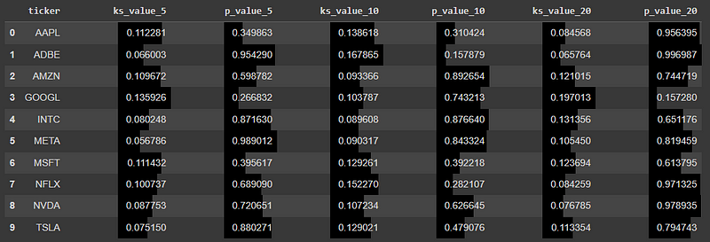
Upon closer inspection of the results, several trends emerged across different tickers and timeframes:
- AAPL: There was no significant deviation from the normal distribution across all three timeframes (5, 10, and 20 days), with p-values above the standard 0.05 threshold.
- ADBE: For the 10-day timeframe, the p-value of 0.157879 indicates a near departure from normality, but the 5 and 20-day returns seem to conform more closely to a normal distribution.
- GOOGL: The 20-day timeframe presents a noticeable departure from a normal distribution with a p-value of 0.157280. However, for shorter durations (5 and 10 days), the returns do not significantly deviate from normality.
- NFLX: The 10-day timeframe, with a p-value of 0.282107, borders on the edge of the typical significance level, suggesting a potential departure from normality. Yet, for 5 and 20 days, the returns adhere more closely to the normal distribution.
The other stocks, such as AMZN, INTC, META, MSFT, NVDA, and TSLA, consistently showed p-values above the 0.05 threshold for all timeframes, indicating that their returns did not significantly deviate from a normal distribution.
These nuanced results demonstrate the intricate nature of stock return distributions and emphasize the importance of adopting a granular, tailored approach in statistical analysis, especially when informing investment decisions.
Conclusion
Our in-depth exploration of stock return distributions using the Shapiro-Wilk test highlighted that many stock returns deviate from the expected Gaussian distribution. Such insights aren’t just academic; they pose practical challenges to foundational principles underlying many financial strategies.
Further depth was added with the Kolmogorov-Smirnov test. This test, being more versatile, brought to light distinct distribution patterns across various stocks. For instance, while stocks like AAPL and AMZN generally conformed to the normal distribution, GOOGL and ADBE showed potential deviations over certain periods.
It’s pivotal to understand the distinction between the two tests. The Shapiro-Wilk test is lauded for its sensitivity and is ideal for determining if a sample stems from a normally distributed population. In contrast, the KS test can be employed against any distribution, making it a versatile tool.
In summation, our research accentuates the necessity of a meticulous, data-driven approach in stock market analysis. There’s no universal solution, and a methodical, individualized analysis is indispensable for investors seeking clarity in the ever-evolving stock market landscape.
Acknowledgments
I sincerely thank everyone who took the time to read and engage with this work. Your curiosity and interest are highly appreciated.
A Message from InsiderFinance

Thanks for being a part of our community! Before you go:
- 👏 Clap for the story and follow the author 👉
- 📰 View more content in the InsiderFinance Wire
- 📚 Take our FREE Masterclass
- 📈 Discover Powerful Trading Tools


