Stock Analysis with a Momentum Strategy

This article delves into the art of predicting stock prices using a momentum-based strategy. The motivation behind this article is a trip down memory lane as I revisit some of the projects from my “AI for Trading” course at Udacity.

Introduction

Analyzing stock markets has always been a challenging and intriguing domain. With the integration of Artificial Intelligence and Machine Learning techniques, this area has seen significant advancements in the last decade. One popular method is based on the momentum strategy, where the main premise is “buying high, selling higher.” Today, we’ll explore this strategy, integrating data acquisition, simulation, metrics calculation, and visualization.

Fetching Stock Data

Before diving deep, let’s talk about our data source. We utilize the yfinance library to extract daily stock data from Yahoo Finance. With this, we can extract the closing prices of our target stocks for the past five years. In this instance, our watchlist includes industry giants like Apple (AAPL), Amazon (AMZN), Microsoft (MSFT), and seven others.

def fetch_stock_data(ticker_list, years=5):
    end_date = datetime.now()
    start_date = end_date - timedelta(days=years * 365)
    stock_data = pd.DataFrame()
    
    for ticker in ticker_list:
        stock = yf.Ticker(ticker)
        hist_data = stock.history(period='1d', start=start_date, end=end_date)
        close_data = hist_data['Close'].rename(ticker)
        stock_data = pd.merge(stock_data, pd.DataFrame(close_data), left_index=True, right_index=True, how='outer')
    return stock_data

# Fetch the data
ticker_list = ['AAPL', 'AMZN', 'MSFT', 'GOOGL', 'META', 'TSLA', 'NVDA', 'ADBE', 'NFLX', 'INTC']
years = 5
daily_data = fetch_stock_data(ticker_list, years)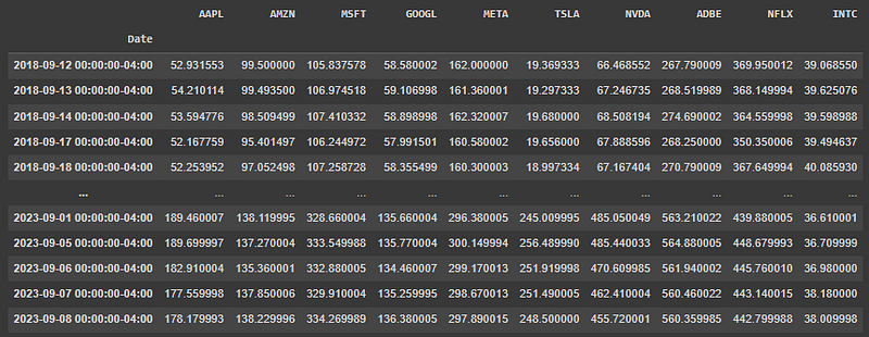

Momentum Strategy Simulation

After obtaining the stock data, our next task is to develop a momentum strategy simulation. This model will:

Resample the stock data according to the desired frequency: daily, weekly, or monthly.
Identify the top-performing stocks based on past log returns.
Allocate funds to these stocks and simulate the portfolio’s performance over time, accounting for potential taxes on gains.

# Resample data to different frequencies: daily, weekly, monthly
def resample_data(data, period):
    if period == 'D':
        return data
    elif period == 'W':
        return data.resample('W').last()
    elif period == 'M':
        return data.resample('M').last()

# Simulate a simple momentum strategy based on log returns
def simulate_momentum_strategy(data, initial_amount, top_n, tax_rate, period='M'):
    data = resample_data(data, period)
    log_returns = np.log(data / data.shift(1))
    simulation_details = pd.DataFrame(index=log_returns.index,
                                      columns=['Selected Stocks', 'Profit Before Tax', 'Tax Paid', 'Portfolio Value'])
    cash = initial_amount

    # Logic to select top stocks and calculate portfolio value
    for i in range(0, len(log_returns) - 1):
        # Identify the top_n performing stocks based on past log returns
        top_stocks = log_returns.iloc[i].sort_values(ascending=False).head(top_n)
        # Filter out stocks with negative returns
        top_stocks = top_stocks[top_stocks > 0]

        if not top_stocks.empty:
            simulation_details.loc[log_returns.index[i + 1], 'Selected Stocks'] = json.dumps(top_stocks.index.tolist())
            # Calculate the amount to allocate for each stock
            num_stocks = len(top_stocks)
            allocation_per_stock = cash / num_stocks
            # Calculate new portfolio value based on the next day's returns
            new_value = sum(allocation_per_stock * np.exp(log_returns.loc[log_returns.index[i + 1], stock]) for stock in top_stocks.index)
            # Calculate and deduct tax if there is a profit
            profit = new_value - cash
            simulation_details.loc[log_returns.index[i + 1], 'Profit Before Tax'] = round(profit, 2)

            if profit > 0:
                tax = profit * tax_rate
                new_value -= tax
                simulation_details.loc[log_returns.index[i + 1], 'Tax Paid'] = round(tax, 2)
            simulation_details.loc[log_returns.index[i + 1], 'Portfolio Value'] = round(new_value, 2)

        else:
            # No allocation, so portfolio value remains the same
            simulation_details.loc[log_returns.index[i + 1], 'Portfolio Value'] = cash
        # Update cash amount for the next round
        cash = simulation_details.loc[log_returns.index[i + 1], 'Portfolio Value']
    # Assign the initial amount to the first row
    simulation_details.loc[log_returns.index[0], 'Portfolio Value'] = initial_amount
    return simulation_details

# Configuration for the momentum strategy simulation
initial_amount = 100000
top_n = 3
tax_rate = 0.15
frequency = 'M'
simulation_details = simulate_momentum_strategy(daily_data, initial_amount, top_n, tax_rate, frequency)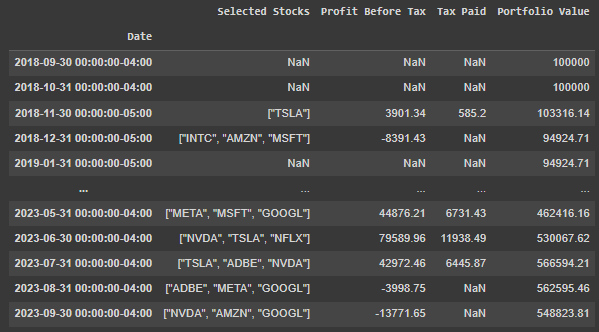

Tracking Individual Investments and Baseline

The momentum strategy is just one of many approaches to stock market investment. While this strategy capitalizes on following asset trends, another approach involves investing a fixed sum in individual stocks, monitoring their performance over time. Furthermore, a prevalent strategy is to evenly distribute investments across desired assets. In this experiment, I’ve established this evenly-distributed approach as the “Baseline”. This portfolio’s value is calculated as the average position of the other assets over each period. In essence, it represents an equal investment in all assets at the start of the period.

# Simulate how each individual stock would have performed over the same period
def track_individual_investments(data, initial_amount, simulation_details, period='W'):
    # Resample data based on the specified period
    data = resample_data(data, period)
    # Calculate returns based on the resampled data
    returns = data.pct_change()
    # Create a new DataFrame to store individual stock values over time
    individual_investments = pd.DataFrame(index=data.index, columns=data.columns)
    for stock in data.columns:
        # Simulate an investment in each stock
        individual_investments[stock] = (1 + returns[stock]).cumprod() * initial_amount
    # Include the Portfolio Value from the momentum strategy
    individual_investments['Portfolio Value'] = simulation_details['Portfolio Value']
    individual_investments['Baseline'] = individual_investments.iloc[:, :-1].T.mean()
    # Adjust the first values to match the Initial Amount.
    individual_investments.iloc[0, :] = initial_amount
    return individual_investments.fillna(0).astype(int)

individual_investments_df = track_individual_investments(daily_data, initial_amount, simulation_details, frequency)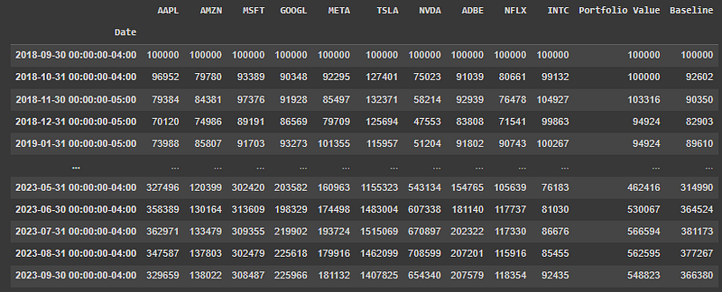

Dataframe View: individual_investments_df

Performance Metrics

To evaluate the efficacy of our investment approach, we employ essential metrics, comparing them against a well-recognized stock market benchmark. Let’s elaborate on the rationale behind this choice:

We’ve opted to use a 10% annual rate as our benchmark in the t-test. This decision is grounded on the historical average return of the S&P 500 index. As reported by NerdWallet, the average stock market return has been about 10% per year for nearly the last century. By using this figure, we aim to contextualize our strategy’s performance against a widely accepted and established market average.

With this decision in mind, here’s a breakdown of the metrics we employ:

Sharpe Ratio:

This metric offers insight into the risk-adjusted performance of an investment, balancing returns against associated risks. Our calculate_sharpe_ratio function adjusts the risk-free rate based on the investment's frequency (daily, weekly, or monthly) to compute this ratio.

T-Test & p-value:

The t_test_portfolio_returns function utilizes a t-test to ascertain if the portfolio's returns deviate significantly from the 10% benchmark rate.

p-value: It represents the likelihood that our portfolio’s returns and the benchmark rate originate from the same statistical distribution. In this context, we halve the p-value, converting it from a two-tailed to a one-tailed test, focusing on the direction of our strategy’s deviation from the benchmark rate. A smaller p-value (typically below 0.05) indicates our strategy’s returns significantly differ from the 10% rate. In our study, a low p-value would affirm the effectiveness of our investment strategy compared to the traditional annual return of 10%.

Overall Portfolio Metrics:

The calculate_metrics function amalgamates all these measures, yielding the final values of each investment, relative growth, annualized mean returns, Sharpe ratios, and the t-statistic along with the p-value. This provides a comprehensive view of our portfolio's performance.

from scipy.stats import ttest_1samp

def calculate_sharpe_ratio(returns, annual_risk_free_rate=0.01, frequency='D'):
    # Adjust the risk-free rate based on the frequency
    if frequency == 'D':
        adjusted_rfr = (1 + annual_risk_free_rate) ** (1/252) - 1
    elif frequency == 'W':
        adjusted_rfr = (1 + annual_risk_free_rate) ** (1/52) - 1
    elif frequency == 'M':
        adjusted_rfr = (1 + annual_risk_free_rate) ** (1/12) - 1

    excess_returns = returns - adjusted_rfr
    return excess_returns.mean() / excess_returns.std()

def t_test_portfolio_returns(portfolio_returns, bench_annual_rate=0.1, frequency='D'):
    # Adjust the risk-free rate based on the frequency
    if frequency == 'D':
        adjusted_rfr = (1 + bench_annual_rate) ** (1/252) - 1
    elif frequency == 'W':
        adjusted_rfr = (1 + bench_annual_rate) ** (1/52) - 1
    elif frequency == 'M':
        adjusted_rfr = (1 + bench_annual_rate) ** (1/12) - 1

    t_stat, p_value = ttest_1samp(portfolio_returns[1:], adjusted_rfr)  # [1:] to exclude the NaN from pct_change
    return t_stat, p_value

def calculate_metrics(dataframe, initial_amount, bench_annual_rate, frequency='D'):
    # Calculate the final and relative values
    final_values = dataframe.iloc[-1]
    relative_values = final_values / initial_amount - 1  # Subtract 1 to get the growth proportion

    # Calculate mean return and Sharpe Ratio
    returns = dataframe.pct_change()

    if frequency == 'D':
        annualization_factor = 252
    elif frequency == 'W':
        annualization_factor = 52
    elif frequency == 'M':
        annualization_factor = 12

    # Corrected annualization of mean returns
    mean_returns = (1 + returns.mean()) ** annualization_factor - 1
    sharpes = returns.apply(calculate_sharpe_ratio, annual_risk_free_rate=0.01, frequency=frequency)

    # Test if the portfolio returns are greater than the adjusted risk-free rate
    portfolio_returns = dataframe['Portfolio Value'].pct_change()
    t_stat, p_value = t_test_portfolio_returns(portfolio_returns, bench_annual_rate, frequency=frequency)

    return final_values, relative_values, mean_returns, sharpes, t_stat, p_value / 2

bench_annual_rate = 0.1

# Calculate the metrics
final_values, relative_values, mean_returns, sharpes, t_stat, p_value = calculate_metrics(individual_investments_df, initial_amount, bench_annual_rate, frequency)

Visualization: Painting the Picture

Utilizing the Plotly library, our investment results are dynamically displayed, presenting the Portfolio Value’s evolution over time and key statistics such as T-test and P-value. Additionally, comparative bar charts provide insights into final investment values, relative growth, annualized Sharpe ratios, and mean returns, offering a consolidated snapshot of the strategy’s performance and effectiveness.

import plotly.graph_objects as go
from plotly.subplots import make_subplots

def plot_combined_charts(dataframe, final_values, relative_values, sharpes, mean_returns):
    labels = final_values.index
    colors = ['#636EFA', '#EF553B', '#00CC96', '#AB63FA', '#FFA15A']

    fig = make_subplots(rows=3, cols=2,
                        subplot_titles=('Portfolio Value Over Time',
                                        '',
                                        'Final Investment Values',
                                        'Relative Investment Growth',
                                        'Annualized Sharpe Ratios',
                                        'Annualized Mean Returns'),
                        vertical_spacing=0.08)

    # Portfolio Value line chart
    fig.add_trace(go.Scatter(x=dataframe.index,
                             y=dataframe['Portfolio Value'],
                             mode='lines',
                             name='Portfolio Value',
                             line=dict(color=colors[0], width=2.5)),
                  row=1, col=1)

    # T-test and P-value
    significance_text = f"<b>T-test:</b> {t_stat:.2f}<br><b>P-value:</b> {p_value:.5f}"
    if t_stat > 2 and p_value < 0.05:
        significance_text += f"<br><b>Significantly different from {bench_annual_rate:.0%} per year!</b>"

    fig.add_annotation(
        text=significance_text,
        showarrow=False,
        xref="x2", yref="y2",
        x=0.5, y=0.5,
        font=dict(size=15),
        bgcolor="white",
        align="center"
    )

    # Final values
    fig.add_trace(go.Bar(x=labels,
                         y=final_values.values,
                         name='Final Values ($)',
                         text=[f"${v:,.2f}" for v in final_values.values],
                         textposition='outside',
                         marker_color=colors[1]),
                  row=2, col=1)

    # Relative Growth
    fig.add_trace(go.Bar(x=labels,
                         y=relative_values.values,
                         name='Relative Growth',
                         text=[f"{v:.2%}" for v in relative_values.values],
                         textposition='outside',
                         marker_color=colors[2]),
                  row=2, col=2)

    # Sharpe Ratios
    fig.add_trace(go.Bar(x=labels,
                         y=sharpes.values,
                         name='Annualized Sharpe Ratio',
                         text=[f"{v:.2f}" for v in sharpes.values],
                         textposition='outside',
                         marker_color=colors[3]),
                  row=3, col=1)

    # Mean Returns
    fig.add_trace(go.Bar(x=labels,
                         y=mean_returns.values,
                         name='Annualized Mean Returns',
                         text=[f"{v:.2%}" for v in mean_returns.values],
                         textposition='outside',
                         marker_color=colors[4]),
                  row=3, col=2)

    # Update layout
    fig.update_layout(title_text="Investment Results Overview",
                      title_font=dict(size=24, color='black', family="Arial Black"),
                      title_pad=dict(t=10),
                      showlegend=False,
                      height=1500,
                      title_x=0.5,
                      bargap=0.05,
                      )

    fig.show()

plot_combined_charts(individual_investments_df, final_values, relative_values, sharpes, mean_returns)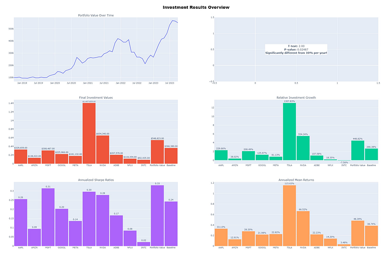

Conclusion

By integrating Artificial Intelligence techniques with trading strategies, the potential becomes evident. During our study, the momentum strategy proved promising. However, it’s essential to highlight the limitations of this article, which can serve as a foundation for subsequent studies:

Fixed Period: Limited to five years, results may vary over different durations.
Fixed Assets: Concentrating on giants like Apple and Amazon, diversifying could change the outcomes.
Market Favorability: The current market benefited the momentum strategy, which may not be consistent in all scenarios.

Lastly, it’s crucial to remember that this article serves more as an introduction to the topic than a thorough validation. In future studies, testing different approaches, varying the number of assets in the portfolio, changing the observation period (from monthly to weekly or even daily), including a variety of new assets across different sizes and sectors, etc., may lead to extraordinary results. Going further, generating overall performance statistics to infer a better strategy is also an exciting path to explore. The possibilities are endless.

Acknowledgments

I sincerely thank everyone who took the time to read and engage with this work. Your curiosity and interest are highly appreciated.

A Message from InsiderFinance

Thanks for being a part of our community! Before you go:

👏 Clap for the story and follow the author 👉
📰 View more content in the InsiderFinance Wire
📚 Take our FREE Masterclass
📈 Discover Powerful Trading Tools