Optimize Portfolio Performance with Risk Parity Rebalancing in Python

Implementation and Evaluation using Key Rolling Risk Metrics

1. Introduction

Instead of merely allocating assets based on potential returns or market capitalization, Risk Parity emphasizes creating a harmonious balance where each asset contributes equally to a portfolio’s overall risk. The goal? Deliver consistent returns while taming the unruly beast of market volatility.

Traditionally, many investors favored a 60/40 stock-bond split for a balanced growth and security blend. However, as financial markets grew more complex, the appeal of sophisticated strategies like Risk Parity surged. This method ensures that each asset, or its group, equally influences the portfolio’s overall risk, preventing disproportionate sway.

1.1 Risk Parity in the Real World

The theoretical appeal of Risk Parity is undeniable, but its real-world applications further cement its reputation in the investment community. A few prominent instances include:

Institutional Adoption: Major financial institutions, including giants like Bridgewater Associates, have integrated Risk Parity in their core funds. They use this strategy to optimize returns and capital preservation, upholding their fiduciary duties to clients.
ETFs and Mutual Funds: Passive investment vehicles like the Invesco Balanced-Risk Allocation Fund and the Wealthfront Risk Parity Fund exemplify the broader accessibility of the Risk Parity strategy. These offerings enable individual investors to tap into an approach previously reserved for institutions, fortifying their portfolios with a refined risk balance.

Risk Parity, with its emphasis on holistic risk management, offers a compelling answer to this age-old conundrum. In the sections that follow, we’ll delve deeper into the mathematical underpinnings of Risk Parity, its Python-based implementation, and further insights into its application, performance, and potential future.

2. Understanding Risk Parity

Risk Parity is an investment approach where the goal is to allocate capital based on risk, rather than on returns or other criteria. The primary objective is to achieve a balanced portfolio where each asset contributes equally to the overall risk. By doing this, the strategy seeks to enhance portfolio diversification and, ideally, achieve more consistent returns over time.

2.1 Conceptual Framework

At its core, Risk Parity is about balance. Traditional investment strategies often rely on expected returns to determine asset allocation, but this can lead to concentrated risks in certain assets. For instance, even in a diversified portfolio, equities might represent a disproportionate amount of risk, especially when market conditions are volatile.

2.2 Mathematical Underpinnings

Volatility as a Measure of Risk: Volatility, often represented by the standard deviation of returns, acts as the primary risk metric in the Risk Parity approach. The higher the volatility of an asset, the greater the risk it carries.
Inverse Volatility Weights: The fundamental formula behind Risk Parity’s allocation strategy is the concept of inverse volatility weighting. Here’s how it works:

The formula for calculating the inverse volatility weights in Risk Parity

Where:

wi is the weight of the asset i,
σi is the volatility of the asset i,
N is the total number of assets in the portfolio.

Simply put, assets with lower volatility are given higher portfolio weights, and vice versa. The goal is to balance out the risk contributions of each asset:

Visualizing the Journey to Risk Parity: as Individual stock risk contributions adjust dynamically, observe how the total portfolio volatility responds in tandem, showcasing the essence of risk balanced asset allocation.

2.3 Benefits and Limitations

Risk Parity isn’t a magic bullet, and like all strategies, it has its strengths and potential pitfalls. On the upside, it provides a more balanced portfolio, potentially leading to steadier returns, especially during tumultuous market periods. On the flip side, the strategy might require the use of leverage to achieve desired returns, which can amplify both gains and losses.

3. Python Implementation

This section will illustrate how one can utilize Python to fetch stock data, compute Risk Parity weights, simulate a Risk Parity portfolio, and visualize the performance results.

3.1. Prerequisites and Libraries

Before we jump into the code, ensure you have the required libraries installed. Our analysis leans on a few essential Python packages:

# Fetch stock data directly from Yahoo Finance.
import yfinance as yf 

# For data manipulation and analysis.
import pandas as pd  

# Used for mathematical operations.
import numpy as np 

# Essential for data visualization.
import matplotlib.pyplot as plt

3.2. Data Fetching

Our starting point is to acquire the historical data for our selected assets and a benchmark index:

def fetch_returns(tickers):
    data = yf.download(tickers + ['^GSPC'], start="2010-01-01", end="2023-01-01")['Adj Close']
    return data.pct_change().dropna()

Here, fetch_returns fetches the adjusted closing prices for our tickers and the S&P 500 (our benchmark), calculates daily returns, and cleans up any NA values.

3.3. Calculating Risk Parity Weights

The essence of Risk Parity lies in balancing risk contributions across assets:

def calculate_weights(data):
    vol = data.rolling(window=60).std().dropna().iloc[-1][:-1]  # Exclude S&P 500 index
    inv_vol = 1 / vol
    weights = inv_vol / np.sum(inv_vol)
    return weights

In calculate_weights, we calculate the rolling 60-day volatility for each asset, derive the inverse volatilities, and normalize them to obtain the Risk Parity weights.

3.4. Portfolio Simulation

Simulating the Risk Parity portfolio’s performance over time:

def simulate_portfolio(returns, n_days=60):
    port_val = [1]
    sp500_val = [1]
    weights = np.ones(len(tickers)) / len(tickers)  # Start with equal weights

    for i in range(len(returns)):
        if i < 60:  # If less than rolling window, use equal weights
            daily_port_return = np.dot(returns.iloc[i][:-1], weights)
        else:
            if i % n_days == 0:  # Rebalancing
                weights = calculate_weights(returns.iloc[i-60:i])
            daily_port_return = np.dot(returns.iloc[i][:-1], weights)

        port_val.append(port_val[-1] * (1 + daily_port_return))
        sp500_val.append(sp500_val[-1] * (1 + returns.iloc[i]['^GSPC']))
    return port_val, sp500_val

The function begins with an equal weightage for all assets. As the simulation progresses, it recalculates the weights based on the Risk Parity principle every n_days. This dynamic adjustment ensures the portfolio remains balanced in terms of risk.

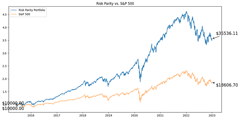
3.5. Comparing Risk Parity to Benchmark

The purpose of any investment strategy is to outperform a benchmark:

def plot_results(returns, port_val, sp500_val):
    plt.figure(figsize=(14, 7))
    plt.plot(returns.index, port_val[:-1], label='Risk Parity Portfolio')
    plt.plot(returns.index, sp500_val[:-1], label='S&P 500', alpha=0.6)
    plt.legend()
    plt.title('Risk Parity vs. S&P 500')

    # Annotations for initial and final values
    initial_val = 10000
    final_rp = port_val[-2] * initial_val  # port_val[-2] because we have an extra entry in port_val list
    final_sp500 = sp500_val[-2] * initial_val  # same reason here

    plt.annotate(f"${initial_val:.2f}", (returns.index[0], port_val[0]), 
                 xytext=(-60,0), textcoords="offset points",
                 arrowprops=dict(arrowstyle="->"), fontsize=15)
    plt.annotate(f"${final_rp:.2f}", (returns.index[-1], port_val[-2]), 
                 xytext=(15,15), textcoords="offset points",
                 arrowprops=dict(arrowstyle="->"), fontsize=15)
    plt.annotate(f"${initial_val:.2f}", (returns.index[0], sp500_val[0]), 
                 xytext=(-60,-20), textcoords="offset points",
                 arrowprops=dict(arrowstyle="->"), fontsize=15)
    plt.annotate(f"${final_sp500:.2f}", (returns.index[-1], sp500_val[-2]), 
                 xytext=(15,-15), textcoords="offset points",
                 arrowprops=dict(arrowstyle="->"), fontsize=15)

    plt.show()

This visualization function plots the performance of our Risk Parity portfolio against the S&P 500. The annotations provide a concise snapshot of the initial investment and the final value, visually demonstrating the portfolio’s growth trajectory.

In the main execution:

tickers = ...
returns = fetch_returns(tickers)
port_val, sp500_val = simulate_portfolio(returns, n_days=30)
plot_results(returns, port_val, sp500_val)

3.6. Complete Code

Portfolio Weights

import yfinance as yf
import pandas as pd
import numpy as np
import matplotlib.pyplot as plt

def fetch_data(tickers):
    data = yf.download(tickers + ['^GSPC'], start="2010-01-01", end="2023-01-01")['Adj Close']
    return data

def calculate_weights(data):
    returns = data.pct_change().dropna()
    vol = returns.rolling(window=60).std().mean()[:-1]  # Exclude S&P 500 index
    inv_vol = 1 / vol
    weights = inv_vol / np.sum(inv_vol)
    return weights * 100  # Convert to percentage

def plot_weights(weights):
    plt.figure(figsize=(12,6))
    weights_sorted = weights.sort_values()
    ax = weights_sorted.plot(kind='barh', color='skyblue')
    plt.title('Risk Parity Weights (%)')
    plt.xlabel('Weights (%)')
    plt.ylabel('Tickers')
    
    # Adding labels to the bars
    for i, v in enumerate(weights_sorted):
        ax.text(v , i, f"{v:.2f}%", va='center', fontweight='light', fontsize=15)
    
    plt.tight_layout()
    plt.show()

# Main
tickers = ['AAPL', 'MSFT', 'AMZN', 'META', 'GOOGL', 'GOOG', 'TSLA', 'BRK-B', 'NVDA', 'JPM', 
           'JNJ', 'V', 'PG', 'UNH', 'MA', 'DIS', 'HD', 'PYPL', 'BAC', 'CMCSA']
data = fetch_data(tickers)
weights = calculate_weights(data)
plot_weights(weights)

Performance Evaluation

import yfinance as yf
import pandas as pd
import numpy as np
import matplotlib.pyplot as plt

def fetch_returns(tickers):
    data = yf.download(tickers + ['^GSPC'], start="2010-01-01", end="2023-01-01")['Adj Close']
    return data.pct_change().dropna()

def calculate_weights(data):
    vol = data.rolling(window=60).std().dropna().iloc[-1][:-1]  # Exclude S&P 500 index
    inv_vol = 1 / vol
    weights = inv_vol / np.sum(inv_vol)
    return weights

def simulate_portfolio(returns, n_days=60):
    port_val = [1]
    sp500_val = [1]
    weights = np.ones(len(tickers)) / len(tickers)  # Start with equal weights

    for i in range(len(returns)):
        if i < 60:  # If less than rolling window, use equal weights
            daily_port_return = np.dot(returns.iloc[i][:-1], weights)
        else:
            if i % n_days == 0:  # Rebalancing
                weights = calculate_weights(returns.iloc[i-60:i])
            daily_port_return = np.dot(returns.iloc[i][:-1], weights)

        port_val.append(port_val[-1] * (1 + daily_port_return))
        sp500_val.append(sp500_val[-1] * (1 + returns.iloc[i]['^GSPC']))
    return port_val, sp500_val

def plot_results(returns, port_val, sp500_val):
    plt.figure(figsize=(14, 7))
    plt.plot(returns.index, port_val[:-1], label='Risk Parity Portfolio')
    plt.plot(returns.index, sp500_val[:-1], label='S&P 500', alpha=0.6)
    plt.legend()
    plt.title('Risk Parity vs. S&P 500')

    # Annotations for initial and final values
    initial_val = 10000
    final_rp = port_val[-2] * initial_val  # port_val[-2] because we have an extra entry in port_val list
    final_sp500 = sp500_val[-2] * initial_val  # same reason here

    plt.annotate(f"${initial_val:.2f}", (returns.index[0], port_val[0]), 
                 xytext=(-60,0), textcoords="offset points",
                 arrowprops=dict(arrowstyle="->"), fontsize=15)
    plt.annotate(f"${final_rp:.2f}", (returns.index[-1], port_val[-2]), 
                 xytext=(15,15), textcoords="offset points",
                 arrowprops=dict(arrowstyle="->"), fontsize=15)
    plt.annotate(f"${initial_val:.2f}", (returns.index[0], sp500_val[0]), 
                 xytext=(-60,-20), textcoords="offset points",
                 arrowprops=dict(arrowstyle="->"), fontsize=15)
    plt.annotate(f"${final_sp500:.2f}", (returns.index[-1], sp500_val[-2]), 
                 xytext=(15,-15), textcoords="offset points",
                 arrowprops=dict(arrowstyle="->"), fontsize=15)

    plt.show()

# Main
tickers = ['AAPL', 'MSFT', 'AMZN', 'META', 'GOOGL', 'GOOG', 'TSLA', 'BRK-B', 'NVDA', 'JPM', 
           'JNJ', 'V', 'PG', 'UNH', 'MA', 'DIS', 'HD', 'PYPL', 'BAC', 'CMCSA']
returns = fetch_returns(tickers)
port_val, sp500_val = simulate_portfolio(returns, n_days=30)
plot_results(returns, port_val, sp500_val)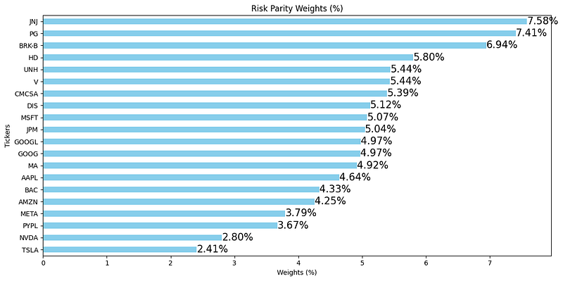

The first visualization depicts the calculated risk parity weights for 20 US equities, highlighting the allocation percentages for optimized risk contribution. Transitioning from the weightage, the second chart contrasts the growth of a risk parity portfolio against the performance of the S&P 500 over time, accentuating the rebalancing effect and its implications on total return.

3.7. Rolling Risk Measures

Performance analysis of the Risk Parity strategy is incomplete without examining the portfolio’s behavior over the investment horizon, especially when juxtaposed against the S&P 500. Here, we’ll visualize three essential aspects: rolling volatility, rolling Sharpe ratio, and asset weight evolution over time.

import matplotlib.gridspec as gridspec

# Calculate rolling metrics 
rolling_vol_rp = pd.Series(port_val[:-1]).pct_change().rolling(window=60).std()
rolling_vol_sp = returns['^GSPC'].rolling(window=60).std()
rolling_sharpe_rp = pd.Series(port_val[:-1]).pct_change().rolling(window=60).mean() / rolling_vol_rp
rolling_sharpe_sp = returns['^GSPC'].rolling(window=60).mean() / rolling_vol_sp

# Calculate weights over time
weights_df = pd.DataFrame(index=returns.index, columns=tickers)
for i, date in enumerate(returns.index):
    if i < 60:
        weights_df.loc[date] = np.ones(len(tickers)) / len(tickers)
    elif i % 60 == 0:
        weights_df.loc[date] = calculate_weights(returns.iloc[i-60:i])
    else:
        weights_df.loc[date] = weights_df.iloc[i-1]

# Create subplots
fig = plt.figure(figsize=(15, 12))
gs = gridspec.GridSpec(3, 1, height_ratios=[1,1,2]) 

# Plot rolling volatility
ax0 = plt.subplot(gs[0])
ax0.plot(returns.index, rolling_vol_rp, label='Risk Parity Rolling Volatility')
ax0.plot(returns.index, rolling_vol_sp, label='S&P 500 Rolling Volatility', alpha=0.6)
ax0.legend()
ax0.set_title('Rolling Volatility')

# Plot rolling Sharpe ratio
ax1 = plt.subplot(gs[1])
ax1.plot(returns.index, rolling_sharpe_rp, label='Risk Parity Rolling Sharpe Ratio')
ax1.plot(returns.index, rolling_sharpe_sp, label='S&P 500 Rolling Sharpe Ratio', alpha=0.6)
ax1.legend()
ax1.set_title('Rolling Sharpe Ratio')

# Plot asset weights over time
ax2 = plt.subplot(gs[2])
weights_df.plot(kind='area', stacked=True, ax=ax2, legend=False)
ax2.legend(loc='center left', bbox_to_anchor=(1, 0.5))
ax2.set_title('Asset Weights Over Time')

plt.tight_layout()
plt.show()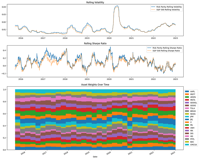

The visualizations provide a three-tiered exploration of portfolio management. The top chart displays the 60-day rolling volatility for both the risk parity portfolio and the S&P 500, offering insights into risk fluctuations over time. The middle section showcases the rolling Sharpe Ratio, highlighting the risk-adjusted returns of the two portfolios. At the base, an area chart illuminates the evolving asset allocation in the risk parity strategy of periodic rebalancing for risk management.

By analyzing these metrics, one can discern that for roughly the same amount of risk, the Risk Parity strategy offers twice as much returns compared to the conventional benchmark! The visual contrast between the portfolio’s rolling volatility and the S&P 500, coupled with the Sharpe ratio, offers an illuminating perspective on the quality and stability of returns.

4. Risk Parity in Diverse Market Conditions

Risk Parity stands out for its risk-balancing emphasis, especially when assessing its performance across market conditions:

4.1. Bull Markets

During bullish periods, equity-centric portfolios naturally shine, with stocks generally offering higher returns. However, Risk Parity, while not overly aggressive, captures a share of this growth. Its risk-focused approach means it might not always maximize on all bullish opportunities, but its strength lies in a more controlled participation.

4.2. Bear Markets

In downturns, the protective nature of Risk Parity becomes evident. With its adaptive rebalancing, the strategy can move away from plummeting assets, favoring safer havens. This can translate to lower drawdowns compared to traditional portfolios.

4.3. Economic Shifts

In both inflationary and deflationary times, Risk Parity’s dynamic allocation adapts to capitalize on the most favorable asset classes.

4.4. Global Impacts

Given global interconnectedness, Risk Parity’s diversification minimizes the effects of major worldwide events.

5. Criticisms and Concerns

As with any investment strategy, Risk Parity is not without its critics. Here, we lay out some of the concerns and counterarguments regarding the approach.

5.1. Dependence on Leverage

Risk Parity often involves using leverage, especially when bonds or other low-volatility assets dominate the portfolio. Critics argue that leverage can amplify losses in turbulent times, potentially negating the benefits of risk balancing.

5.2. Complexity and Costs

The dynamic nature of Risk Parity can lead to frequent rebalancing, which might result in higher transaction costs. Additionally, understanding the nuances of the strategy might be challenging for retail investors without a financial background.

5.3. Over-reliance on Quantitative Models

While quantitative models form the backbone of the Risk Parity strategy, relying solely on them can be risky. Models are as good as the assumptions they’re based on. Unprecedented market events can throw a spanner in the works, leading to unexpected results.

6. Future Prospects for Risk Parity

The financial world is ever-evolving, and strategies must adapt or risk becoming obsolete. Here’s a peek into the future of Risk Parity:

6.1. Incorporation of Alternative Assets

To diversify risk further, there’s an increasing trend toward including alternative assets like real estate, commodities, or even cryptocurrencies in Risk Parity portfolios.

6.2. Advent of AI and Machine Learning

Advanced algorithms can offer predictive insights, potentially refining the Risk Parity strategy. By forecasting macroeconomic shifts or understanding intricate asset correlations better, AI and machine learning might drive the next evolution in Risk Parity investing.

6.3. Broader Adoption by Retail Investors

With the advent of financial technology and easy-to-use investment platforms, complex strategies like Risk Parity could become more accessible to the average investor.

Concluding Remarks

Risk Parity stands out as a methodological approach, aiming to harness the power of diversified risk rather than diversified assets. As we’ve seen, it’s not merely a theoretical concept but has found practical application in the real world, from large institutions to retail investors’ portfolios.

However, as with any strategy, it’s essential to approach Risk Parity with a discerning mind. Its merits are evident in its historical performance and its ability to weather various market conditions, but it’s not without its criticisms. Investors considering this strategy should weigh its potential rewards against its inherent complexities and risks.