Free AI web copilot to create summaries, insights and extended knowledge, download it at here
8201
Abstract
-comment"># defining a data frame to store portfolio returns</span>
portfolio_strategy_returns = pd.DataFrame()
portfolio_bnh_returns = pd.DataFrame()
<span class="hljs-comment"># buy and hold returns for individual stocs</span>
bnh_stock_returns = []
bnh_stock_sharpe = []
<span class="hljs-comment"># iterating over stocks in the portfolio</span>
<span class="hljs-keyword">for</span> stock <span class="hljs-keyword">in</span> portfolio_stocks:
data = get_daily_data(stock, start, end)
<span class="hljs-comment"># Calculating daily returns</span>
data[<span class="hljs-string">"bnh_returns"</span>] = np.log(data[<span class="hljs-string">"Close"</span>]/data[<span class="hljs-string">"Close"</span>].shift())
portfolio_strategy_returns[stock] = ma(data,ma1 = <span class="hljs-number">10</span>, ma2 = <span class="hljs-number">25</span>)
bnh_stock_returns.append(get_cumulative_return(data[<span class="hljs-string">"strategy_returns"</span>]))
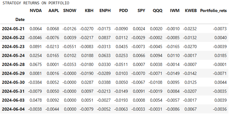
bnh_stock_sharpe.append(get_annualized_sharpe_ratio(data[<span class="hljs-string">"strategy_returns"</span>]))</pre></div><ul><li>Printing the SMA strategy returns</li></ul><div id="c7fc"><pre><span class="hljs-built_in">print</span>(<span class="hljs-string">"\nSTRATEGY RETURNS ON PORTFOLIO"</span>)
portfolio_strategy_returns[<span class="hljs-string">"Portfolio_rets"</span>] = portfolio_strategy_returns.mean(axis=<span class="hljs-number">1</span>)
portfolio_strategy_returns.<span class="hljs-built_in">round</span>(decimals = <span class="hljs-number">4</span>).tail(<span class="hljs-number">10</span>)</pre></div><figure id="9d01"><img src="https://cdn-images-1.readmedium.com/v2/resize:fit:800/1*uI6K6ZXoWxLSwkoaooTerQ.png"><figcaption>STRATEGY RETURNS ON PORTFOLIO</figcaption></figure><ul><li>Calculating cumulative returns and the annualized Sharpe ratio</li></ul><div id="b235"><pre>perf = pd.DataFrame(index=portfolio_stocks,columns=[<span class="hljs-string">"Cumulative returns"</span>,<span class="hljs-string">"Annualized Sharpe Ratio"</span>])
<span class="hljs-keyword">for</span> i,stock <span class="hljs-keyword">in</span> <span class="hljs-built_in">enumerate</span>(portfolio_stocks):
cum_ret = bnh_stock_returns[i]
anu_shp = bnh_stock_sharpe[i]
perf.loc[stock] = [cum_ret,anu_shp]
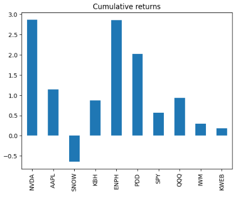
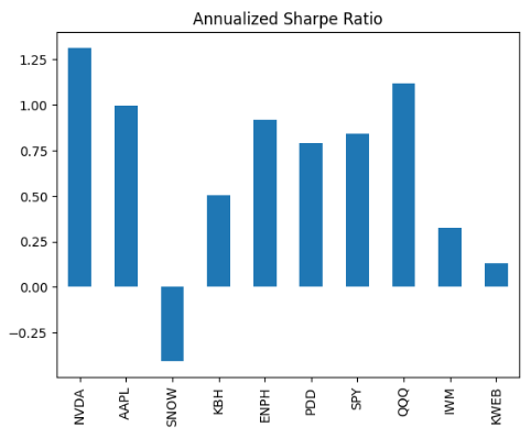
perf
Cumulative returns Annualized Sharpe Ratio
NVDA <span class="hljs-number">2.375256</span> <span class="hljs-number">1.071783</span>
AAPL <span class="hljs-number">1.176463</span> <span class="hljs-number">1.020626</span>
SNOW -<span class="hljs-number">0.110298</span> -<span class="hljs-number">0.068875</span>
KBH <span class="hljs-number">0.839733</span> <span class="hljs-number">0.482885</span>
ENPH <span class="hljs-number">2.455573</span> <span class="hljs-number">0.784543</span>
PDD <span class="hljs-number">2.237751</span> <span class="hljs-number">0.900318</span>
SPY <span class="hljs-number">0.592832</span> <span class="hljs-number">0.886599</span>
QQQ <span class="hljs-number">0.637886</span> <span class="hljs-number">0.746084</span>
IWM <span class="hljs-number">0.213217</span> <span class="hljs-number">0.233466</span>
KWEB <span class="hljs-number">0.549323</span> <span class="hljs-number">0.404803</span></pre></div><ul><li>Comparing the Stock Cumulative Returns</li></ul><div id="96d8"><pre>perf[<span class="hljs-string">'Cumulative returns'</span>].plot.bar(title=<span class="hljs-string">'Cumulative returns'</span>)</pre></div><figure id="d303"><img src="https://cdn-images-1.readmedium.com/v2/resize:fit:800/1*TnGcb1YxZ5ChXCLbcLYqzw.png"><figcaption>Stock Cumulative Returns</figcaption></figure><ul><li>Comparing the Stock Annualized Sharpe Ratio</li></ul><div id="cbb3"><pre>perf[<span class="hljs-string">'Annualized Sharpe Ratio'</span>].plot.bar(title=<span class="hljs-string">'Annualized Sharpe Ratio'</span>)</pre></div><figure id="9680"><img src="https://cdn-images-1.readmedium.com/v2/resize:fit:800/1*O8SRFclHvcr36uPp7YuYmw.png"><figcaption>Stock Annualized Sharpe Ratio</figcaption></figure><ul><li>Calculating the stock performance mean value</li></ul><div id="935a"><pre>perf.mean()
Cumulative returns <span class="hljs-number">1.096774</span>
Annualized Sharpe Ratio <span class="hljs-number">0.646223</span>
dtype: <span class="hljs-built_in">object</span></pre></div><ul><li>Calculating the SMA strategy cumulative return and the annualized Sharpe ratio</li></ul><div id="879d"><pre><span class="hljs-built_in">print</span>(<span class="hljs-string">"Cumulative returns SMA Strategy :"</span>,get_cumulative_return(portfolio_strategy_returns[<span class="hljs-string">"Portfolio_rets"</span>]))
<span class="hljs-built_in">print</span>(<span class="hljs-string">"Annualized sharpe ratio SMA Strategy :"</span>,get_annualized_sharpe_ratio(portfolio_strategy_returns[<span class="hljs-string">"Portfolio_rets"</span>]))
Cumulative returns SMA Strategy : <span class="hljs-number">1.17530067503038</span>
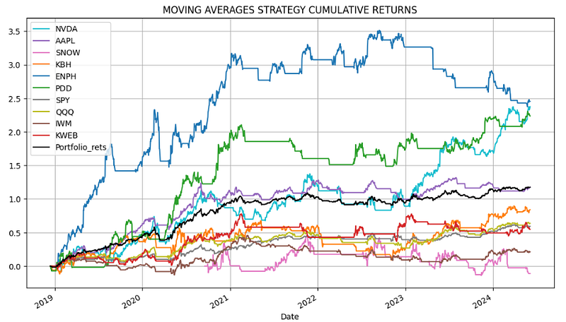
Annualized sharpe ratio SMA Strategy : <span class="hljs-number">1.2276872946556154</span></pre></div><ul><li>We can see that the SMA strategy results in ROI ~ 17.5%, and the annualized Sharpe ratio from 1 to 1.99 is considered adequate/good.</li><li>Plotting and comparing the SMA strategy cumulative returns</li></ul><div id="53e3"><pre><span class="hljs-keyword">import</span> matplotlib.pyplot <span class="hljs-keyword">as</span> plt
colors = [<span class="hljs-string">'tab:cyan'</span>,<span class="hljs-string">'tab:purple'</span>,<span class="hljs-string">'tab:pink'</span>,<span class="hljs-string">'tab:orange'</span>,<span class="hljs-string">'tab:blue'</span>,<span class="hljs-string">'tab:green'</span>,<span class="hljs-string">'tab:gray'</span>,<span class="hljs-string">'tab:olive'</span>,<span class="hljs-string">'tab:brown'</span>,<span class="hljs-string">'tab:red'</span>,<span class="hljs-string">"k"</span>]
portfolio_strategy_returns.cumsum().plot(figsize=(<span class="hljs-number">12</span>,<span class="hljs-number">7</span>), title=<span class="hljs-string">"MOVING AVERAGES STRATEGY CUMULATIVE RETURNS"</span>, color=colors)
plt.grid()</pre></div><figure id="a158"><img src="https://cdn-images-1.readmedium.com/v2/resize:fit:800/1*NdXscvvjAMCM_4gaBkdRrA.png"><figcaption>SMA strategy cumulative returns (step 1).</figcaption></figure><ul><li>Let’s move to step 2 by excluding the worst performer SNOW with the lowest cumulative return and the negative annualized Sharpe ratio (a Sharpe ratio less than 1 is considered bad).</li></ul><h2 id="6707">Step 2: Excluding Worst Performers with Lowest Returns</h2><ul><li>Applying the above sequence to the updated portfolio of 9 assets without SNOW</li></ul><div id="e972"><pre><span class="hljs-comment"># portfolio of stocks</span>
portfolio_stocks = [<span class="hljs-string">"NVDA"</span>,<span class="hljs-string">"AAPL"</span>,<span class="hljs-string">"KBH"</span>,<span class="hljs-string">"ENPH"</span>,<span class="hljs-string">"PDD"</span>,<span class="hljs-string">"SPY"</span>,<span class="hljs-string">"QQQ"</span>,<span class="hljs-string">"IWM"</span>,<span class="hljs-string">"KWEB"</span>]</pre></div><ul><li>Calculating the stock performance mean value</li></ul><div id="af02"><pre>perf.mean()
Cumulative returns <span class="hljs-number">1.300106</span>
Annualized Sharpe Ratio <span class="hljs-number">0.767578</span>
dtype: <span class="hljs-built_in">object</span></pre></div><ul><li>Calculating the SMA strategy cumulative return and the annualized Sharpe ratio</li></ul><div id="5e92"><pre><span class="hljs-built_in">print</span>(<span class="hljs-string">"Cumulative returns SMA Strategy :"</span>,get_cumulative_return(portfolio_strategy_returns[<span class="hljs-string">"Portfolio_rets"</span>]))
<span class="hljs-built_in">print</span>(<span class="hljs-string">"Annualized sharpe ratio SMA Strategy :"</span>,get_annualized_sharpe_ratio(portfolio_strategy_returns[<span class="hljs-string">"Portfolio_rets"</span>]))
Cumula
Options
tive returns SMA Strategy : <span class="hljs-number">1.3001058358012645</span>
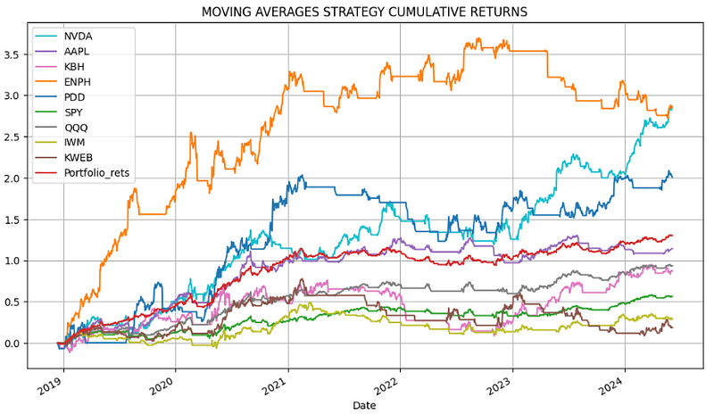
Annualized sharpe ratio SMA Strategy : <span class="hljs-number">1.3648948755238106</span></pre></div><ul><li>We can see that the updated SMA strategy yields ROI ~ 30% and the improved annualized Sharpe ratio of 1.365.</li><li>Plotting and comparing the SMA strategy cumulative returns</li></ul><figure id="ea61"><img src="https://cdn-images-1.readmedium.com/v2/resize:fit:800/1*dv9mtGZT0-ejzNz-S1X-TA.png"><figcaption>SMA strategy cumulative returns (step 2).</figcaption></figure><ul><li>Let’s move to step 3 by thresholding the poor performers KWEB, IWM and SPY with the cumulative returns <0.6.</li></ul><h2 id="e5df">Step 3: Excluding Poor Performers with Lowest Sharpe Ratio</h2><ul><li>Applying the above sequence to the updated portfolio of 6 assets without SNOW, KWEB, IWM and SPY, viz.</li></ul><div id="e754"><pre><span class="hljs-comment"># portfolio of stocks</span>
portfolio_stocks = [<span class="hljs-string">"NVDA"</span>,<span class="hljs-string">"AAPL"</span>,<span class="hljs-string">"KBH"</span>,<span class="hljs-string">"ENPH"</span>,<span class="hljs-string">"PDD"</span>,<span class="hljs-string">"QQQ"</span>]</pre></div><ul><li>Calculating the stock performance mean value</li></ul><div id="cbbb"><pre>perf.mean()
Cumulative returns <span class="hljs-number">1.776673</span>
Annualized Sharpe Ratio <span class="hljs-number">0.936473</span>
dtype: <span class="hljs-built_in">object</span></pre></div><ul><li>Calculating the SMA strategy cumulative return and the annualized Sharpe ratio</li></ul><div id="8b7d"><pre><span class="hljs-built_in">print</span>(<span class="hljs-string">"Cumulative returns SMA Strategy :"</span>,get_cumulative_return(portfolio_strategy_returns[<span class="hljs-string">"Portfolio_rets"</span>]))
<span class="hljs-built_in">print</span>(<span class="hljs-string">"Annualized sharpe ratio SMA Strategy :"</span>,get_annualized_sharpe_ratio(portfolio_strategy_returns[<span class="hljs-string">"Portfolio_rets"</span>]))
Cumulative returns SMA Strategy : <span class="hljs-number">1.7766732115541535</span>
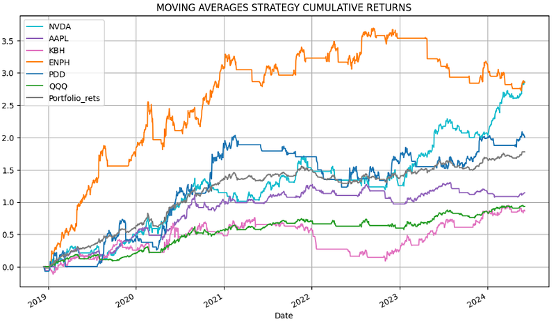
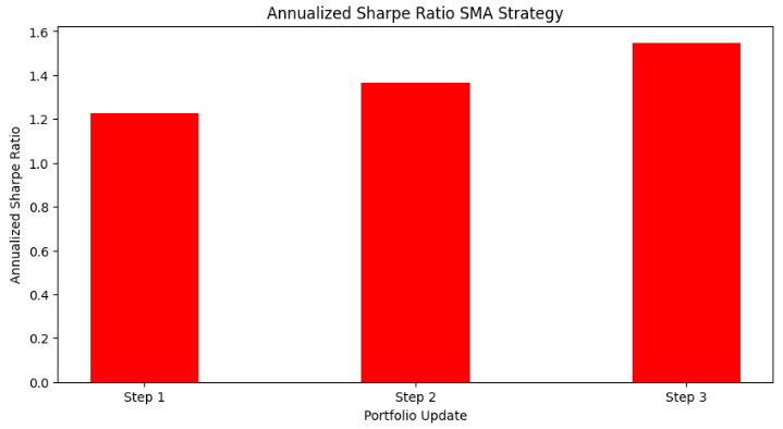
Annualized sharpe ratio SMA Strategy : <span class="hljs-number">1.5475252825461494</span></pre></div><ul><li>We can see that the updated SMA strategy yields ROI ~ 77.6% and the improved annualized Sharpe ratio of ~1.55 (significantly closer to the very good value of 2 than other two portfolios).</li><li>Plotting and comparing the SMA strategy cumulative returns</li></ul><figure id="6d1f"><img src="https://cdn-images-1.readmedium.com/v2/resize:fit:800/1*5hH04HJMoUMDBiPchyIV2A.png"><figcaption>SMA strategy cumulative returns (step 3).</figcaption></figure><h2 id="ecc5">Conclusions</h2><ul><li>Here is the visual summary of our three updates towards the optimal portfolio:</li></ul><div id="0b0e"><pre><span class="hljs-comment"># creating the dataset</span>
data = {<span class="hljs-string">'Step 1'</span>:<span class="hljs-number">1.227</span>, <span class="hljs-string">'Step 2'</span>:<span class="hljs-number">1.365</span>, <span class="hljs-string">'Step 3'</span>: <span class="hljs-number">1.547</span>}
courses = <span class="hljs-built_in">list</span>(data.keys())
values = <span class="hljs-built_in">list</span>(data.values())
fig = plt.figure(figsize = (<span class="hljs-number">10</span>, <span class="hljs-number">5</span>))
<span class="hljs-comment"># creating the bar plot</span>
plt.bar(courses, values, color =<span class="hljs-string">'red'</span>,
width = <span class="hljs-number">0.4</span>)
plt.xlabel(<span class="hljs-string">"Portfolio Update"</span>)
plt.ylabel(<span class="hljs-string">"Annualized Sharpe Ratio"</span>)
plt.title(<span class="hljs-string">"Annualized Sharpe Ratio SMA Strategy"</span>)
plt.show()</pre></div><figure id="296b"><img src="https://cdn-images-1.readmedium.com/v2/resize:fit:800/1*Fs_UIEwSLNO-u3_Wki1bnw.png"><figcaption>Annualized Sharpe Ratio SMA Strategy</figcaption></figure><div id="fef2"><pre><span class="hljs-comment"># creating the dataset</span>
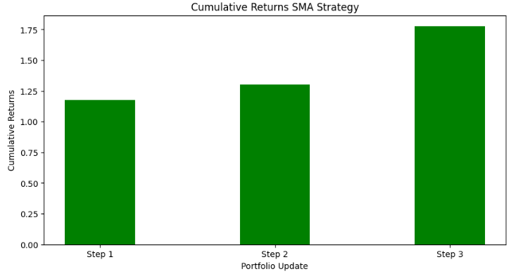
data = {<span class="hljs-string">'Step 1'</span>:<span class="hljs-number">1.175</span>, <span class="hljs-string">'Step 2'</span>:<span class="hljs-number">1.300</span>, <span class="hljs-string">'Step 3'</span>: <span class="hljs-number">1.776</span>}
courses = <span class="hljs-built_in">list</span>(data.keys())
values = <span class="hljs-built_in">list</span>(data.values())
fig = plt.figure(figsize = (<span class="hljs-number">10</span>, <span class="hljs-number">5</span>))
<span class="hljs-comment"># creating the bar plot</span>
plt.bar(courses, values, color =<span class="hljs-string">'green'</span>,
width = <span class="hljs-number">0.4</span>)
plt.xlabel(<span class="hljs-string">"Portfolio Update"</span>)
plt.ylabel(<span class="hljs-string">"Cumulative Returns"</span>)
plt.title(<span class="hljs-string">"Cumulative Returns SMA Strategy"</span>)
plt.show()</pre></div><figure id="e5e0"><img src="https://cdn-images-1.readmedium.com/v2/resize:fit:800/1*jAogfMJTZdnmZaDTNAliyQ.png"><figcaption>Cumulative Returns SMA Strategy</figcaption></figure><ul><li>In summary, this IPO project intended to investigate the ability of proposed SMA portfolio updates to assist investors to make profitable trading decisions.</li><li>Our backtesting experiments show that the proposed workflow can maximize risk-adjusted returns of portfolios while minimizing the number of assets involved in the optimization process.</li><li>Our Road Ahead in Portfolio Management is to combine advanced trading strategies, financial health/risk metrics and stochastic portfolio optimization algorithms into a single framework to optimize the advantages of each.</li></ul><h2 id="cbbc">Explore More</h2><ul><li><a href="https://wp.me/pdMwZd-4Je">Portfolio Optimization of 20 Dividend Growth Stocks</a></li><li><a href="https://wp.me/pdMwZd-4IB">Towards Max(ROI/Risk) Trading</a></li><li><a href="https://wp.me/pdMwZd-371">XOM SMA-EMA-RSI Golden Crosses ‘22</a></li><li><a href="https://wp.me/pdMwZd-7A3">Plotly Dash TA Stock Market App</a></li><li><a href="https://wp.me/pdMwZd-2f2">Bear vs. Bull Portfolio Risk/Return Optimization QC Analysis</a></li><li><a href="https://wp.me/pdMwZd-1D2">Towards min(Risk/Reward) — SeekingAlpha August Bear Market Update</a></li></ul><h2 id="11a3">References</h2><ul><li><a href="https://blog.devgenius.io/algorithmic-trading-backtesting-portfolio-of-stocks-in-python-9be75ce9f232">Algorithmic Trading — Backtesting Portfolio of Stocks in Python</a></li><li><a href="https://readmedium.com/maximizing-profitability-of-moving-average-crossover-trading-strategy-what-moving-averages-to-use-e5cd70085690">Maximizing Profitability of Moving Average Crossover Trading Strategy: What moving averages to use?</a></li><li><a href="https://www.pythonforfinance.net/2017/01/28/optimisation-of-moving-average-crossover-trading-strategy-in-python/">OPTIMIZATION OF MOVING AVERAGE CROSSOVER TRADING STRATEGY IN PYTHON</a></li><li><a href="https://www.investopedia.com/articles/active-trading/052014/how-use-moving-average-buy-stocks.asp">How to Use a Moving Average to Buy Stocks</a></li><li><a href="https://www.investopedia.com/investing/how-renew-and-adjust-your-portfolio/">How To Adjust and Renew Your Portfolio</a></li><li><a href="https://www.youtube.com/watch?v=wJmXMboLE64">How to beat the Market. Momentum and Portfolio Optimization</a></li><li><a href="https://www.fmz.com/lang/en/strategy/439870">Moving Average Crossover Trading Strategy</a></li><li><a href="https://www.quantstart.com/static/ebooks/sat/sample.pdf">Strategy Optimization</a></li></ul><h2 id="9308">Contacts</h2><ul><li><a href="https://newdigitals.org/">Website</a></li><li><a href="https://github.com/alva922">GitHub</a></li><li><a href="https://twitter.com/alzapress">X/Twitter</a></li><li><a href="https://nl.pinterest.com/alexzap922/">Pinterest</a></li><li><a href="https://mastodon.social/@alexzap">Mastodon</a></li><li><a href="https://alva922.tumblr.com/">Tumblr</a></li></ul></article></body>