Maximizing Profitability of Moving Average Crossover Trading Strategy: What moving averages to use?

As traders, we are always searching for the best trading strategies that will maximize profitability while minimizing risks. The dual moving average crossover trading strategy is a popular and straightforward technique that uses two moving averages to predict market trends and entry/exit points.
To implement this strategy, we first calculate the short-term and long-term moving averages of the price of a security. These moving averages can be of different lengths and are mathematically designed to have different variances and rates of direction. When the two moving averages intersect or “cross over,” it is a signal to buy or sell the security.
The technical approach to this strategy suggests that when the short-term moving average (STMA) crosses above the long-term moving average (LTMA), it is a signal to buy or go long. Conversely, when the STMA crosses below the LTMA, it is a signal to sell or go short. This approach is based on the principle of momentum, which states that a price moving up or down in period t is likely to continue moving in the same direction in period t+1.
In this article, we will discuss how to maximize profitability with the dual moving average crossover trading strategy by exploring the different moving average combinations that traders can use. By choosing the right moving average lengths, traders can optimize their strategy and improve their chances of success.
The basic strategy
First, we import the libraries that we going to use for the analysis:
import numpy as np
import pandas as pd
import yfinance as yf

import matplotlib.pyplot as plt
import plotly.graph_objs as go
import seaborn as sns
We useyfinance (imported as yf), a library allowing easy access to Yahoo Finance’s financial data. With yfinance, you can download historical market data for stocks, options, and currencies.
#Download ticker price data from yfinance
tick = 'ARKK'
ticker = yf.Ticker(tick)
ticker_history = ticker.history(period='10y')
For this example, we analyze 10 years of the daily price history of ARKK, the ticker of ARK Innovation ETF but feel free to use other securities.
#Calculate 10 and 20 days moving averages
ticker_history['ma10'] = ticker_history['Close'].rolling(window=10).mean()
ticker_history['ma20'] = ticker_history['Close'].rolling(window=20).mean()

#Create a column with buy and sell signals
ticker_history['signal'] = 0.0
ticker_history['signal'] = np.where(ticker_history['ma10'] > ticker_history['ma20'], 1.0, 0.0)

#Calculate daily returns for the ticker
ticker_history['returns'] = ticker_history['Close'].pct_change()

#Calculate strategy returns
ticker_history['strategy_returns'] = ticker_history['signal'].shift(1) * ticker_history['returns']

#Calculate cumulative returns for the ticker and the strategy
ticker_history['cumulative_returns'] = (1 + ticker_history['returns']).cumprod()
ticker_history['cumulative_strategy_returns'] = (1 + ticker_history['strategy_returns']).cumprod()

#Print the cumulative strategy returns at the last date
ticker_history['cumulative_strategy_returns'][-1]
2.690754730303438
This indicates that the result of the strategy in the period analyzed is 269.075%. In the same period, a Buy and Hold strategy would have had a return of 203.12%
We can create a chart with the cumulative returns for the ticker and the strategy applied with Plotly.
fig = go.Figure()
fig.add_trace(go.Scatter(x=ticker_history.index, y=ticker_history['cumulative_returns'], name=tick,
                         line=dict(color='white', width=2)))
fig.add_trace(go.Scatter(x=ticker_history.index, y=ticker_history['cumulative_strategy_returns'], name='Estrategy',
                         line=dict(color='#22a7f0', width=2)))
fig.update_layout(title=('Moving average crossover strategy backtest in ' + tick),
                  xaxis_title='Date',
                  yaxis_title='Cumulative performance',
                  font=dict(color='white'),
                  paper_bgcolor='black',
                  plot_bgcolor='black',
                  legend=dict(x=0, y=1.2, bgcolor='rgba(0,0,0,0)'),
                  yaxis=dict(gridcolor='rgba(255,255,255,0.2)'),
                  xaxis=dict(gridcolor='rgba(255,255,255,0.2)'))
fig.update_xaxes(showgrid=True, ticklabelmode="period")
fig.update_yaxes(showgrid=True)
fig.show()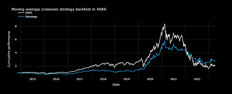
But performance is not the only important thing, we can also analyze the drawdown of the strategy.
Drawdown is a financial term that refers to the maximum loss an investment portfolio or an asset has experienced from its peak value. It is the difference between the highest point of the investment’s value and the lowest point it reaches before it recovers.
Drawdowns are important because they provide insight into the risk and volatility of an investment. High drawdowns indicate that an investment is more volatile and risky, while low drawdowns suggest a more stable investment. Therefore, understanding drawdowns can help investors manage their portfolios and assess the potential risk and rewards of their investments.
We can study the drawdown of the strategy with the following code:
#Calculate the maximum cumulative returns of the strategy so far
ticker_history['cumulative_strategy_max'] = ticker_history['cumulative_strategy_returns'].cummax()

#Calculate the current drawdown of the strategy returns in relation to the maximum cumulative returns
ticker_history['cumulative_strategy_drawdown'] = (ticker_history['cumulative_strategy_returns'] / ticker_history['cumulative_strategy_max']) - 1

#Print the current drawdown
print('The current drawdown of the strategy is:', ticker_history['cumulative_strategy_drawdown'][-1])
The current drawdown of the strategy is: -0.5364383150776705
But what if we change STMA to 20 and STMA to 40? Or STMA to 9 and STMA to 21? Taking into count that the most common MA are 5, 7, 9, 10, 20, 21, 30, 40, 50, 100, and 200 we can analyze the returns and drawdown of different combination MA.
Returns matrix with different moving averages
In order to create the matrix, first we develop a similar model of MA crossover
#Define base slow and fast moving averages
fast_ma = 10
slow_ma = 20

#Calculate the moving averages for the strategy
ticker_history['fast_ma'] = ticker_history['Close'].rolling(window=fast_ma).mean()
ticker_history['slow_ma'] = ticker_history['Close'].rolling(window=slow_ma).mean()

#Create a column with buy and sell signals
ticker_history['signal'] = np.where(ticker_history['fast_ma'] > ticker_history['slow_ma'], 1.0, 0.0)

# Calculate daily ticker and strategy returns
ticker_history['returns'] = ticker_history['Close'].pct_change()
ticker_history['strategy_returns'] = ticker_history['signal'].shift(1) * ticker_history['returns']
Then, we create a null matrix with different combinations of moving averages using a Pandas DataFrame:
# Define two lists of fast and slow moving average values to be used as index and columns for a returns matrix
fast_ma_range = [5, 7, 9, 10, 20, 21, 30, 40, 50, 100]
slow_ma_range = [7, 9, 10, 20, 21, 30, 40, 50, 100, 200]

# Create a DataFrame with the index and columns as the fast and slow moving average values, respectively
# The DataFrame will be used to store returns data for different combinations of the moving averages
returns_matrix = pd.DataFrame(index=fast_ma_range, columns=slow_ma_range)
As a result, we obtain a null 10x10 matrix. To fill it with the hypothetical returns of strategies with different combinations of MA we use 2 for loops:
# Iterate through all combinations of fast and slow moving average values
for fast_ma in fast_ma_range:
    for slow_ma in slow_ma_range:

        # Calculate the fast and slow moving averages of the stock's closing price
        ticker_history['fast_ma'] = ticker_history['Close'].rolling(window=fast_ma).mean()
        ticker_history['slow_ma'] = ticker_history['Close'].rolling(window=slow_ma).mean()

        # Generate a signal to buy (1.0) or sell (0.0) based on the relative positions of the two moving averages
        ticker_history['signal'] = np.where(ticker_history['fast_ma'] > ticker_history['slow_ma'], 1.0, 0.0)

        # Calculate the daily returns of the stock and the strategy
        ticker_history['strategy_returns'] = ticker_history['signal'].shift(1) * ticker_history['returns']

        # Calculate the cumulative returns of the strategy
        cumulative_strategy_returns = (1 + ticker_history['strategy_returns']).cumprod()

        # Add the cumulative returns of the strategy to the returns matrix
        returns_matrix.loc[fast_ma, slow_ma] = cumulative_strategy_returns[-1]
Now we have a complete matrix with returns of strategies with different combinations of MA. To visualize we can create a heat map using Seaborn library:
# Make a copy of the returns_matrix and convert index and columns to string type
values = returns_matrix.copy()
values.index = values.index.astype(str)
values.columns = values.columns.astype(str)

# Convert values to float type
values = values.astype(float)

# Change the style of the plot and set the default color scheme
plt.style.use('dark_background')
sns.set_palette("bright")

# Create a heatmap with the provided values, including annotations, using the RdYlGn color map
sns.heatmap(values, annot=True, cmap='RdYlGn')

# Add labels to the axes
plt.xlabel('Slow Moving Average', fontsize=12, color='white')
plt.ylabel('Fast Moving Average', fontsize=12, color='white')

# Add a title to the plot
plt.title('Heatmap of Returns', fontsize=16, color='white')

# Increase the font size to 0.8 and change the color to white for all text elements
sns.set(font_scale=0.8, rc={'text.color':'white', 'axes.labelcolor':'white', 'xtick.color':'white', 'ytick.color':'white'})

# Change the background color of the plot to black
fig = plt.gcf()
fig.set_facecolor('#000000')

# Display the plot
plt.show()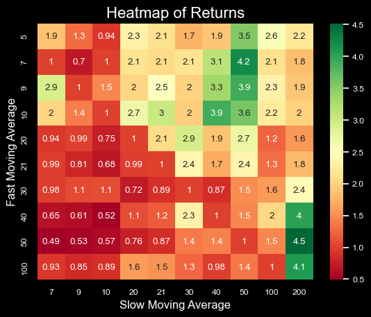
As we can see in the graph above, strategies with different combinations of moving averages can achieve uneven returns. The best 2 combinations for the analyzed period are:
- STMA:50, LTMA:200 with a cumulative return of 4.5 (451.48%)
- STMA:7, LTMA:50 with a cumulative return of 4.2 (421.29%)
200, 50, and 40 seem to be good options to choose as LTMA for this security but is not too clear to choose a good candidate for STMA.
Complementary, we can analyze drawdowns for different combinations of moving averages as we did with returns.
Drawdowns matrix with different moving averages
Create another null matrix with different combinations of moving averages using a Pandas DataFrame:
# Define two lists of fast and slow moving average values to be used as index and columns for a returns matrix
fast_ma_range = [5, 7, 9, 10, 20, 21, 30, 40, 50, 100]
slow_ma_range = [7, 9, 10, 20, 21, 30, 40, 50, 100, 200]

# Create a DataFrame with the index and columns as the fast and slow moving average values, respectively
# The DataFrame will be used to store returns data for different combinations of the moving averages
dd_matrix = pd.DataFrame(index=fast_ma_range, columns=slow_ma_range)
As a result, we obtain a null 10x10 matrix. To fill it with the hypothetical drawdowns of strategies with different combinations of MA we use 2 for loops:
# Loop through different values for fast and slow moving averages
for fast_ma in fast_ma_range:
    for slow_ma in slow_ma_range:

        # Calculate the moving averages for the strategy
        ticker_history['fast_ma'] = ticker_history['Close'].rolling(window=fast_ma).mean()
        ticker_history['slow_ma'] = ticker_history['Close'].rolling(window=slow_ma).mean()

        # Create a binary signal column for buy/sell signals
        ticker_history['signal'] = np.where(ticker_history['fast_ma'] > ticker_history['slow_ma'], 1.0, 0.0)

        # Calculate daily returns for the ticker and the strategy
        ticker_history['strategy_returns'] = ticker_history['signal'].shift(1) * ticker_history['returns']

        # Calculate cumulative returns for the strategy
        ticker_history['cumulative_strategy_returns'] = (1 + ticker_history['strategy_returns']).cumprod()

        # Calculate maximum cumulative returns for the strategy
        ticker_history['cumulative_strategy_max'] = ticker_history['cumulative_strategy_returns'].cummax()

        # Calculate the drawdown for the strategy
        ticker_history['cumulative_strategy_drawdown'] = (ticker_history['cumulative_strategy_returns'] / ticker_history['cumulative_strategy_max']) - 1

        # Add drawdown to the matrix of drawdowns
        dd_matrix.loc[fast_ma, slow_ma] = ticker_history['cumulative_strategy_drawdown'][-1]
Now we have a complete matrix with drawdowns of strategies with different combinations of MA. To visualize we can create a heat map using the Seaborn library:
# Make a copy of the drawdown matrix and convert the index and columns to string type
values_dd = dd_matrix.copy()
values_dd.index = values_dd.index.astype(str)
values_dd.columns = values_dd.columns.astype(str)

# Convert values to float type
values_dd = values_dd.astype(float)

# Change the style of the plot and set the default color scheme
plt.style.use('dark_background')
sns.set_palette("bright")

# Create a heatmap with the provided values, including annotations, using the RdYlGn color map
sns.heatmap(values_dd, annot=True, cmap='RdYlGn')

# Add labels to the axes
plt.xlabel('Slow Moving Average', fontsize=12, color='white')
plt.ylabel('Fast Moving Average', fontsize=12, color='white')

# Add a title to the plot
plt.title('Heatmap of Drawdowns', fontsize=16, color='white')

# Increase the font size to 0.8 and change the color to white for all text elements
sns.set(font_scale=0.8, rc={'text.color':'white', 'axes.labelcolor':'white', 'xtick.color':'white', 'ytick.color':'white'})

# Change the background color of the plot to black
fig = plt.gcf()
fig.set_facecolor('#000000')

# Display the plot
plt.show()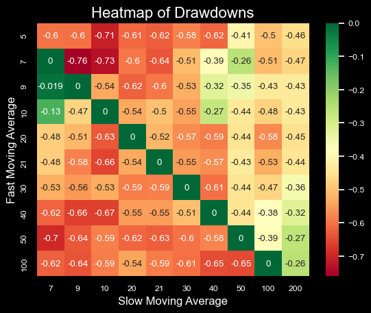
Again, we see positive metrics in strategies that work with 40 and 200 LTMA for this asset. On the other hand, the matrix presents high drawdowns for fast numbers like STMA:5//LTMA:10 or STMA:7//LTMA:9.
Final thoughts
Through the study carried out, it can be observed how the choice of different moving averages can affect the results of the strategy. However, great care must be taken when parameterizing possible strategies since the study shows results on past quotes (see in-sample vs out-of-sample for more info).
In addition, it is very important to take into account that to apply this strategy in a real environment, commissions should be added to the analysis, as well as the effect of slippage. This probably reduces the performance of the strategies, but it would be possible to add other rules such as investing at a risk-free rate when not trading, shorting when a sell signal is observed, etc.
See the complete code in GitHub (Spanish version)