Uncovering Hidden Gems with Multi-Objective Portfolio Optimization: MPT, CAPM, Beta, Vol, Sharpe, PyPortfolioOpt & SciPy


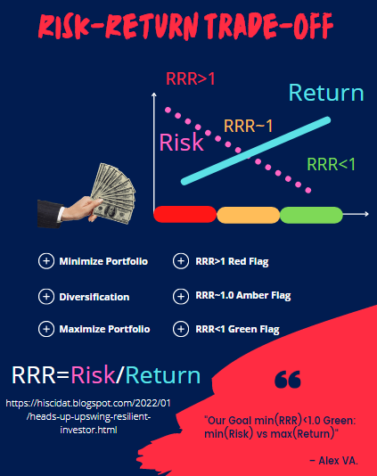
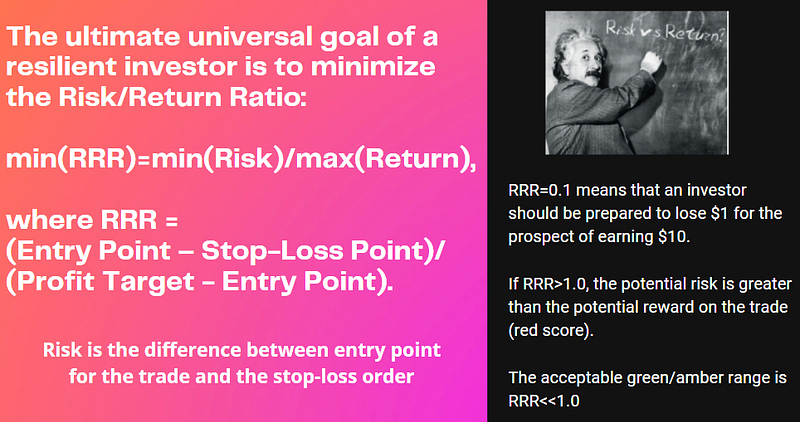
- The subject of this quant trading study is the optimal selection process of financial instruments that maximizes the Return/Risk Ratio (RRR).
- Decision makers in fintech need to make trade-offs between the conflicting objectives. Therefore, it is important that the multiple objectives are to be considered explicitly, including the uncertainties in expected RRR.
- The objective typically maximizes factors such as expected return, and minimizes costs like financial risk, resulting in a multi-objective optimization problem.
- Investment portfolio optimization (IPO) involves using various simulation and multi-parameter minimization scenarios to construct an asset portfolio that geared towards maximizing ROI within given risk boundaries or minimizing risk for a desired level of return.
- In this article, we consider a multi-period IPO problem, which is an extension of the single-period IPO approach.
- Using an investment universe of global stock indices, bonds, and commodities, we test the performance of optimized portfolios and compare the results to the S&P 500 benchmark for multiple periods.
- For example, we may be interested in selecting a few stocks from the listed S&P 500 companies to ensure they make the most profit possible.
- IPO can also help diversify investments whilst minimizing risks. For example, the mean variance IPO may select a portfolio containing assets in tech, retail, healthcare and real estate instead of a single industry like tech.
- Modern Portfolio Theory (MPT) is one of the most popular IPO techniques focused on building portfolios which maximize expected return given a predefine level of risk.
- Here is a practical example of the Python IPO algorithm:
- We generate N random portfolios. That is N portfolios containing our M stocks with different weights (N>>M).
- We calculate portfolio returns, portfolio risk and the Sharpe Ratio for each of the randomly generated assets.
- Then, we visualize the portfolio returns, risks and Sharpe Ratio using Matplotlib, seaborn or Plotly.
- Finally, we determine the optimal portfolio with the highest return, lowest risk and the highest Sharpe Ratio as compared to the S&P benchmark.
- PyPortfolioOpt is a Python library specifically designed to solve IPO problems. It provides efficient algorithms for finding the portfolio with max(RRR) by calculating the efficient frontier.
- Conventionally, the pandas and numpy libraries can be used for handling data and mathematical operations, respectively, while scipy.optimize can be utilized for the optimization process itself.
Project Goals:
- The ultimate goal is to identify and remove low-value assets from a portfolio, or to allocate more budget towards securities that are high value.
- By building a well-diversified portfolio that holds multiple assets and asset classes, we’ll be better positioned to weather volatility and reduce the risk of losing all of our capital.
- We’ll address another key issue in the definition of asset allocation: how to articulate it across different time horizons.
Business Case:
- In today’s competitive, global economy, it is imperative that investors have a well-planned, balanced (growth) portfolio.
- IPO is an important tool to help investors reposition, grow, achieve sustainable long-term profits or get their products ready for sale.
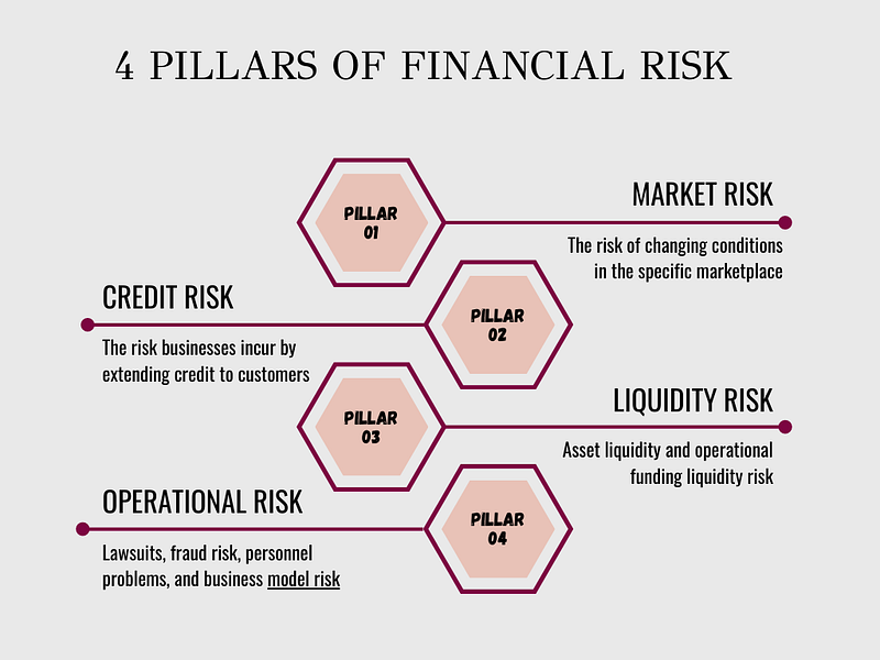
- IPO stands among key enablers of the Risk Intelligent Enterprise, along with risk governance, risk sensing, and scenario planning.
Methods:
- Modern Portfolio Theory
- Mean-Variance Optimization
- Black-Litterman Model
- Monte Carlo Simulation
- Risk Parity
Scope:
- It is all about optimization analysis with constraints and uncertainty bounds. To optimize means to “make the best or most effective use of a situation, opportunity, or resource” (Dictionary.com).
- Virtually every investor has limited resources, and the goal is to generate as much business value (“bang”) with the limited resources available (“the buck”).
- Monte Carlo simulations offer a powerful tool to assess different asset allocation strategies and their potential outcomes under uncertain market conditions.
- We’ll test the performance of various stochastic simulation methods by examining a plethora of well-diversified assets for multiple time horizons.
Theoretical Background:
- The modern portfolio theory (MPT) is a practical method for selecting investments in order to maximize their overall returns within an acceptable level of risk. The MPT can be useful to investors trying to construct efficient and diversified portfolios.
- Among the most prominent approaches to IPO, Mean-Variance Optimization (MVO) pioneered by Markowitz (1952) stands as a cornerstone in MPT. Specifically, we will explore the Markowitz’s Efficient Frontier, a crucial concept that identifies the optimal combination of assets in a portfolio.
- The Black-Litterman (BL) model is an asset allocation tool that portfolio managers use to optimize investor portfolios according to their risk tolerance and market outlook. The model uses market equilibrium as a starting point and considers the investors’ subjective market views to calculate how the optimal asset weights should differ from the initial portfolio allocation. The model attempts to create more stable and efficient portfolios based on investors’ unique insight, which overcomes the issues of input sensitivity.
- Monte Carlo simulations offer a powerful tool to assess different asset allocation strategies and their potential outcomes under uncertain market conditions.
- The risk parity approach to portfolio construction seeks to allocate the capital in a portfolio based on a risk-weighted basis. Asset allocation is the process by which an investor divides the capital in a portfolio among different types of assets. Following the tenets of MPT, this approach makes use of the efficient frontier and security market line (SML) to find the optimal asset allocation.
Some Popular Methods:
- Market Cap Weighted
- Inverse Volatility
- Equal Risk
- Max Diversification & Min Variance
- Mean Variance Optimal.
A Few Challenges
- Typical optimal weights have too large a range.
- The mean return of a security changes due to time and other factors (so do covariances).
- Even if the mean (one-year, say) return is constant over time, it takes decades to get an accurate estimate.
- The optimal weights are sensitive to mean return estimates.
- The optimal weights usually produce disappointing results when used on a real-time, prospective basis.
- Besides, portfolio managers want to use their stock picking “skills.”
Let’s delve into the specifics of out IPO scenario testing aimed at max (RRR)!
Scenario 1: MPT Crypto
Stocks: Top 10 Cryptocurrencies by MC
tickers="BTC-USD ETH-USD USDT-USD USDC-USD BNB-USD BUSD-USD XRP-USD ADA-USD SOL-USD DOGE-USD"Time Horizon: start=”2022–01–03", end=”2024–05–11"
Methods: Monte Carlo
Objectives: Max Sharpe Ratio
Libraries: yfinance
- Let’s begin with cryptocurrency IPO using Markowitz theory. Markowitz put two parameters at the head of his theory — risk and profitability. An efficient frontier is one that defines the effective set of portfolios on it, respectively, between risk and return.
- Here’s the simple hands-on example:
import os
os.chdir('YOURPATH')    # Set working directory
os. getcwd()

# Basic Imports

import yfinance as yf
import numpy as np
import pandas as pd
import os
import seaborn as sns

#Fetching historical crypto data

data = yf.download("BTC-USD ETH-USD USDT-USD USDC-USD BNB-USD BUSD-USD XRP-USD ADA-USD SOL-USD DOGE-USD", start="2022-01-03", end="2024-05-11")

N_iterations = 15000
import matplotlib.pyplot as plt
#calculate percentage change between the current and a prior element - it will be daily returns
daily_returns = data['Adj Close'].pct_change()
num_assets = len(daily_returns.columns)

#calculate covariance matrix
cov_matrix = (daily_returns.cov())*365 # multiply by days in year to get annual covariance

# run optimization of portfolio weights
dict_portfolios = {"portfolio_std":[],"portfolio_returns":[],"weights":[], "sharpe_ratio":[]}
for i in range(N_iterations):

    #get random weights and calculate returns and variance
    weights = np.random.random(num_assets)
    weights = weights/np.sum(weights)
    expected_portfolio_return = np.sum(daily_returns.mean()*weights)
    expected_portfolio_variance = np.dot(weights.T,np.dot(cov_matrix,weights))
    sharpe_ratio = expected_portfolio_return / np.sqrt(expected_portfolio_variance)

    # collect all portfolios in the dictionary
    dict_portfolios['portfolio_std'].append(np.sqrt(expected_portfolio_variance)) # get standard deviation instead of variance
    dict_portfolios['portfolio_returns'].append(expected_portfolio_return)
    dict_portfolios['weights'].append(weights)
    dict_portfolios['sharpe_ratio'].append(sharpe_ratio)

simulated_portfolios=pd.DataFrame(dict_portfolios)

# Plot returns vs. standard deviation to find optimal portfolio (efficient frontier)
simulated_portfolios.plot.scatter(x='portfolio_std', y='portfolio_returns', marker='o', s=10, alpha=0.3, grid=True, figsize=[10,10])
max_sharpe_ratio = simulated_portfolios.query('sharpe_ratio == sharpe_ratio.max()')

# red dot for max sharpe ratio
plt.plot(max_sharpe_ratio['portfolio_std'],max_sharpe_ratio['portfolio_returns'],'ro',markersize=20)
plt.ylabel('Mean daily returns')
plt.xlabel('Annual volatility (standard deviation)')
plt.show()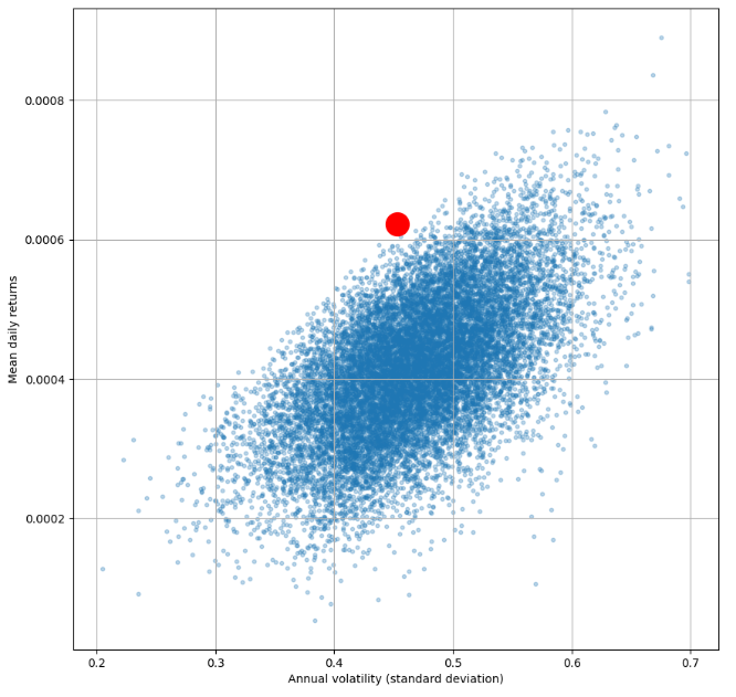
- Checking the portfolio weights
# check the portfolio weights

dictionary_of_weights = {}
for i in range(len(daily_returns.columns)):
    dictionary_of_weights [daily_returns.columns[i]] = max_sharpe_ratio['weights'].values[0][i]
print('max sharpe ratio: \n')
efficient_frontier = pd.DataFrame.from_dict(dictionary_of_weights, orient='index').reset_index()
efficient_frontier.columns = ['crypto pair','weights']
display(efficient_frontier)

max sharpe ratio:

crypto pair weights
0 ADA-USD 0.001532
1 BNB-USD 0.256517
2 BTC-USD 0.113406
3 BUSD-USD 0.104682
4 DOGE-USD 0.031886
5 ETH-USD 0.022788
6 SOL-USD 0.227143
7 USDC-USD 0.225962
8 USDT-USD 0.012950
9 XRP-USD 0.003134- Plotting the portfolio weights
from matplotlib import pyplot as plt
import numpy as np
WIDTH_SIZE=9
HEIGHT_SIZE=9
fig = plt.figure(figsize=(WIDTH_SIZE,HEIGHT_SIZE))
ax = fig.add_axes([0,0,1,1])
ax.axis('equal')
langs = efficient_frontier['crypto pair']
students = efficient_frontier['weights']
ax.pie(students, labels = langs,autopct='%1.2f%%')
plt.show()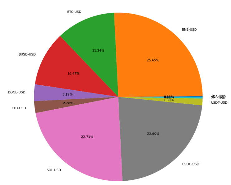
Scenario 2: Energy-Defense-ETF Diversification
Stocks: XOM, LMT, SCHD
Time Horizon: 1Y
Methods: Monte Carlo
Objectives: Max Sharpe Ratio
Libraries: yfinance
import os
os.chdir('YOURPATH')    # Set working directory
os. getcwd()
#BASIC IMPORTS
import pandas as pd
import requests
import numpy as np
import matplotlib.pyplot as plt
from math import floor
from termcolor import colored as cl
import yfinance as yf
from yahoofinancials import YahooFinancials

plt.rcParams['figure.figsize'] = (20, 10)
plt.style.use('fivethirtyeight')- Loading XOM historical data
ticker = yf.Ticker('XOM')
aapl_df = ticker.history(period="1y")
aapl_df['Close'].plot(title="XOM's stock price")
aapl_df.tail()
                           Open       High       Low       Close     Volume Dividends Stock Splits
Date
2024-05-06 00:00:00-04:00 116.669998 118.339996 116.400002 116.750000 31401300 0.0 0.0
2024-05-07 00:00:00-04:00 117.279999 117.580002 115.930000 116.169998 30122000 0.0 0.0
2024-05-08 00:00:00-04:00 115.709999 116.949997 115.410004 116.150002 18957200 0.0 0.0
2024-05-09 00:00:00-04:00 116.199997 118.529999 116.190002 118.440002 17561300 0.0 0.0
2024-05-10 00:00:00-04:00 118.540001 118.650002 117.809998 117.928001 4910616 0.0 0.0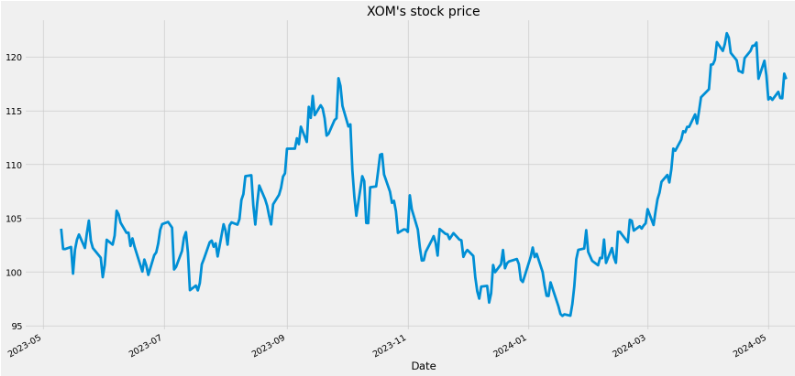
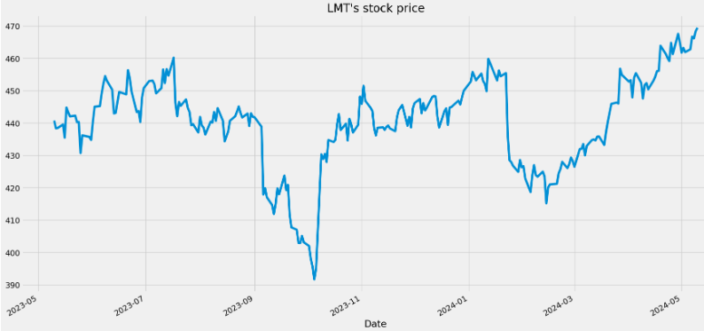
- Loading LMT historical data
ticker = yf.Ticker('LMT')
ibm_df = ticker.history(period="1y")
ibm_df['Close'].plot(title="LMT's stock price")
- Loading SCHD historical data
ticker = yf.Ticker('SCHD')
azn_df = ticker.history(period="1y")
azn_df['Close'].plot(title="SCHD's stock price")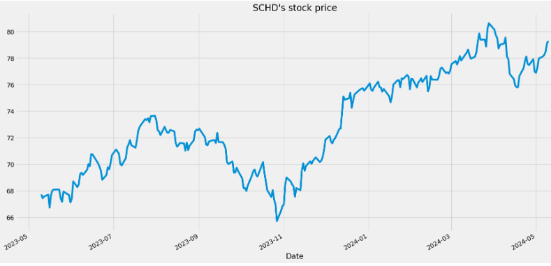
- Normalizing the stock prices and calculating Normed Return
aapl = aapl_df[['Close']]
ibm = ibm_df[['Close']]
azn = azn_df[['Close']]
stock_df=aapl
stock_df['Normed Return'] = stock_df['Close']/ stock_df.iloc[0]['Close']
aapl=stock_df
aapl.tail()
                          Close      Normed Return
Date
2024-05-06 00:00:00-04:00 116.750000 1.122402
2024-05-07 00:00:00-04:00 116.169998 1.116826
2024-05-08 00:00:00-04:00 116.150002 1.116634
2024-05-09 00:00:00-04:00 118.440002 1.138650
2024-05-10 00:00:00-04:00 117.928001 1.133727

stock_df=ibm
stock_df['Normed Return'] = stock_df['Close']/ stock_df.iloc[0]['Close']
ibm=stock_df
ibm.tail()

                          Close     Normed Return
Date
2024-05-06 00:00:00-04:00 462.779999 1.050026
2024-05-07 00:00:00-04:00 466.679993 1.058875
2024-05-08 00:00:00-04:00 466.160004 1.057695
2024-05-09 00:00:00-04:00 468.390015 1.062755
2024-05-10 00:00:00-04:00 469.429993 1.065115

stock_df=azn
stock_df['Normed Return'] = stock_df['Close']/ stock_df.iloc[0]['Close']
azn=stock_df
azn.tail()

                          Close    Normed Return
Date
2024-05-06 00:00:00-04:00 78.129997 1.153580
2024-05-07 00:00:00-04:00 78.250000 1.155352
2024-05-08 00:00:00-04:00 78.510002 1.159191
2024-05-09 00:00:00-04:00 79.160004 1.168788
2024-05-10 00:00:00-04:00 79.279999 1.170560- Assigning the portfolio allocation weights [0.5,0.2,0.3] and the investment amount $100k
for stock_df, allo in zip((aapl, ibm,azn),[0.5,0.2,0.3]):
    stock_df['Allocation'] = stock_df['Normed Return']*allo

for stock_df in (aapl, ibm, azn):
stock_df['Position Amount']= stock_df['Allocation']*100000- Plotting the cumulative return of the entire portfolio vs individual stocks
total_pos_vals = [aapl['Position Amount'], ibm['Position Amount'], azn['Position Amount']]
portf_vals = pd.concat(total_pos_vals, axis = 1)
portf_vals.columns = ['XOM', 'LMT', 'SCHD']
portf_vals['Total Pos'] = portf_vals.sum(axis=1)
portf_vals['Total Pos'].plot(figsize = (10,6))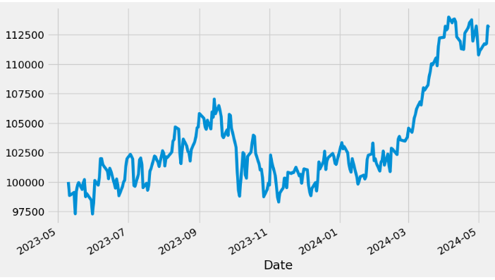
portf_vals['2023-03-01':].drop('Total Pos', axis = 1).plot(figsize=(10,6));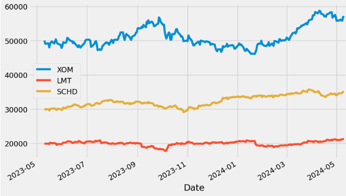
- Calculating the mean portfolio daily return and std
portf_vals['Daily Return'] = portf_vals['Total Pos'].pct_change(1)
portf_vals.dropna(inplace = True)
print('Daily Return Average: ',portf_vals['Daily Return'].mean())
print('Daily Return Standard Deviation: ',portf_vals['Daily Return'].std())

Daily Return Average:  0.0005255601943780237
Daily Return Standard Deviation: 0.008596775975364407- Plotting the density vs histogram of the portfolio daily returns
portf_vals['Daily Return'].plot(kind = 'hist', bins=100, figsize = (6,8), color = 'green')
portf_vals['Daily Return'].plot(kind = 'kde', figsize = (8,6), color = 'r');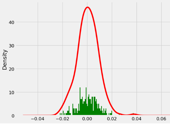
- Calculating the cumulative return of our portfolio
cumulative_return = 100*(portf_vals['Total Pos'][-1]/portf_vals['Total Pos'][0]-1)
print('Cumulative return: ', cumulative_return)
Cumulative return: 14.416636530936788- Calculating the portfolio Sharpe ratio
SR = portf_vals['Daily Return'].mean()/portf_vals['Daily Return'].std()
print('Sharpe Ratio = ', SR)
Sharpe Ratio =  0.06113456903891762
#Annual Sharpe Ratio:
ASR = (252**0.5) * SR
print('Annualized Sharpe Ratio = ', ASR)

Annualized Sharpe Ratio =  0.9704811971165102
- Stock close price preparation for IPO
stocks = pd.concat([aapl['Close'], ibm['Close'], azn['Close']], axis = 1)
stocks.columns = ['XOM', 'LMT', 'SCHD']
stocks.tail()
                          XOM        LMT        SCHD
Date
2024-05-06 00:00:00-04:00 116.750000 462.779999 78.129997
2024-05-07 00:00:00-04:00 116.169998 466.679993 78.250000
2024-05-08 00:00:00-04:00 116.150002 466.160004 78.510002
2024-05-09 00:00:00-04:00 118.440002 468.390015 79.160004
2024-05-10 00:00:00-04:00 117.928001 469.429993 79.279999- Comparing mean stock daily returns
stocks.pct_change(1).mean()
XOM     0.000584
LMT     0.000307
SCHD    0.000650
dtype: float64- Examining the stock daily return correlation matrix
stocks.pct_change(1).corr()
     XOM       LMT     SCHD
XOM 1.000000 0.297715 0.426209
LMT 0.297715 1.000000 0.289254
SCHD 0.426209 0.289254 1.000000

import seaborn as sns
fig, ax = plt.subplots(figsize=(5, 5))
sns.heatmap(stocks.pct_change(1).corr(),ax=ax).set(title='Correlation Matrix')
plt.show()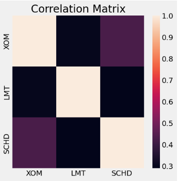
- Comparing the stock log returns histograms
log_returns = np.log(stocks/stocks.shift(1))
log_returns.hist(bins = 100, figsize = (12,8), color = 'g')
plt.tight_layout()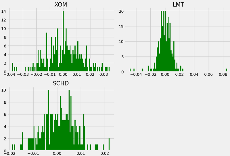
- Calculating and plotting the covariance matrix of stock log returns
log_returns.cov()*252

     XOM     LMT      SCHD
XOM 0.043198 0.010293 0.009932
LMT 0.010293 0.028296 0.005459
SCHD 0.009932 0.005459 0.012576

import seaborn as sns
fig, ax = plt.subplots(figsize=(5, 5))
sns.heatmap(log_returns.cov()*252,ax=ax).set(title='Covariance Matrix')
plt.show()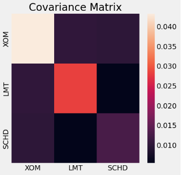
- Choosing an optimal portfolio allocation within the MPT framework
np.random.seed(101)
print(stocks.columns)

weights = np.array(np.random.random(3))

print('Random Weights: ')
print(weights)

#However, their sum must be equal to 100
print('Rebalance')
weights = weights/np.sum(weights)
print(weights)

Index(['XOM', 'LMT', 'SCHD'], dtype='object')
Random Weights:
[0.51639863 0.57066759 0.02847423]
Rebalance
[0.46291341 0.51156154 0.02552505]

exp_ret = np.sum((log_returns.mean() * weights) * 252)
print('Expected Portfolio Return: ',exp_ret)

Expected Portfolio Return:  0.09439096736312266

exp_vol = np.sqrt(np.dot(weights.T,np.dot(log_returns.cov() * 252, weights)))
print('Expected Volatility: ', exp_vol)
Expected Volatility:  0.14806090936894675

SR = exp_ret/exp_vol
print('Sharpe Ratio: ', SR)

Sharpe Ratio:  0.6375144375745645

#Choosing an optimal portfolio allocation.
num_ports = 10000
all_weights = np.zeros((num_ports,len(stocks.columns)))
ret_arr = np.zeros(num_ports)
vol_arr = np.zeros(num_ports)
sharpe_arr = np.zeros(num_ports)

for ind in range(num_ports):
    weights = np.array(np.random.random(3))
    weights = weights / np.sum(weights)
    all_weights[ind,:] = weights
    ret_arr[ind] = np.sum((log_returns.mean() * weights) *252)
    vol_arr[ind] = np.sqrt(np.dot(weights.T, np.dot(log_returns.cov() * 252, weights)))
    sharpe_arr[ind] = ret_arr[ind]/vol_arr[ind]

sharpe_arr.max()
1.4038899601457429

sharpe_arr.argmax()
3761

all_weights[sharpe_arr.argmax(),:]

array([0.01272508, 0.0033809 , 0.98389403])

plt.figure(figsize = (12,8))
plt.scatter(vol_arr,ret_arr,c=sharpe_arr,cmap='Spectral')
plt.colorbar(label='Sharpe Ratio')
plt.xlabel('Volatility')
plt.ylabel('Return')

# Add red dot for max SR
max_sr_ret = ret_arr[sharpe_arr.argmax()]
max_sr_vol = vol_arr[sharpe_arr.argmax()]
plt.scatter(max_sr_vol,max_sr_ret,c='red',s=450,edgecolors='black');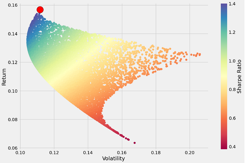
Read More:
- Fin Analysis-Portfolio Allocation Optimization
- Portfolio Optimization: Using Python
- Get Financial Data from Yahoo Finance with Python
- Download Financial Dataset Using Yahoo Finance in Python | A Complete Guide
- Markowitz Portfolio Optimization — Gold and Amazon
Scenario 3: PyPortfolioOpt MPT
Stocks: PFE, WM, DIS, CLX
Time Horizon: 2010–2023
Methods: The Markowitz Mean-Variance Model
Objectives: Testing PyPortfolioOpt Efficient Frontier
Libraries: PyPortfolioOpt
# Setting working directory
import os
os.chdir('YOURPATH')    # Set working directory
os. getcwd()
#Installing pyportfolioopt
!pip install pyportfolioopt
- Preparing input stock data for IPO
import yfinance as yf
# Getting dataframes info for Stocks using yfinance
aapl_df = yf.download('PFE', start = '2010-01-01', end = '2023-04-09')
tsla_df = yf.download('WM', start = '2010-01-01', end = '2023-04-09')
dis_df = yf.download('DIS', start = '2010-01-01', end = '2023-04-09')
amd_df = yf.download('CLX', start = '2010-01-01', end = '2023-04-09')

# Extracting Adjusted Close for each stock
aapl_df = aapl_df['Adj Close']
tsla_df = tsla_df['Adj Close']
dis_df = dis_df['Adj Close']
amd_df = amd_df['Adj Close']

import pandas as pd
# Merging and creating an Adj Close dataframe for stocks
df = pd.concat([aapl_df, tsla_df, dis_df, amd_df], join = 'outer', axis = 1)
df.columns = ['pfe', 'wm', 'dis', 'clx']
df # Visualizing dataframe for input

           pfe       wm        dis       clx
Date
2010-01-04 11.026819 23.771673 27.933918 41.983829
2010-01-05 10.869543 23.667282 27.864237 42.441734
2010-01-06 10.834594 23.660328 27.716160 42.332390
2010-01-07 10.793817 23.716005 27.724873 41.929150
2010-01-08 10.881195 23.827343 27.768423 41.935989
... ... ... ... ...
2023-03-31 40.799999 163.169998 100.129997 158.240005
2023-04-03 41.349998 163.869995 99.760002 156.750000
2023-04-04 40.900002 163.529999 99.570000 155.899994
2023-04-05 41.549999 162.820007 99.910004 157.419998
2023-04-06 41.500000 163.660004 99.970001 157.759995
3338 rows × 4 columns
- Calculating the annualized expected returns and the sample covariance matrix
# Importing libraries for portfolio optimization
import pypfopt
from pypfopt.efficient_frontier import EfficientFrontier
from pypfopt import risk_models
from pypfopt import expected_returns

# Calculating the annualized expected returns and the annualized sample covariance matrix
mu = expected_returns.mean_historical_return(df) #expected returns
S = risk_models.sample_cov(df) #Covariance matrix

# Visualizing the annualized expected returns
mu
pfe    0.105267
wm     0.156843
dis    0.101074
clx    0.105136
dtype: float64

# Visualizing the covariance matrix
S
    pfe      wm       dis      clx
pfe 0.046326 0.017478 0.020015 0.012002
wm  0.017478 0.035693 0.021444 0.014009
dis 0.020015 0.021444 0.068004 0.010278
clx 0.012002 0.014009 0.010278 0.043615- Using Efficient Frontier to maximize the Sharpe ratio
# Optimizing for max Sharpe ratio
ef = EfficientFrontier(mu, S) # Providing expected returns and covariance matrix as input
weights = ef.max_sharpe() # Optimizing weights for Sharpe ratio maximization

clean_weights = ef.clean_weights() # clean_weights rounds the weights and clips near-zeros

# Printing optimized weights and expected performance for portfolio
clean_weights
OrderedDict([('pfe', 0.0841), ('wm', 0.7439), ('dis', 0.0), ('clx', 0.172)])- Creating the new portfolio with optimized weights
new_weights = [0.7439, 0.172]
optimized_portfolio = tsla_df.pct_change()*new_weights[0] + amd_df.pct_change()*new_weights[1]
optimized_portfolio # Visualizing daily returns
Date
2010-01-04         NaN
2010-01-05   -0.001391
2010-01-06   -0.000662
2010-01-07    0.000112
2010-01-08    0.003520
                ...
2023-03-31    0.011785
2023-04-03    0.001572
2023-04-04   -0.002476
2023-04-05   -0.001553
2023-04-06    0.004209
Name: Adj Close, Length: 3338, dtype: float64- Using Efficient Frontier to maximize the Sharpe ratio
import pandas as pd
from pypfopt.efficient_frontier import EfficientFrontier
from pypfopt import risk_models
from pypfopt import expected_returns
# Calculate expected returns and sample covariance
mu = expected_returns.mean_historical_return(df)
S = risk_models.sample_cov(df)
# Optimize for maximal Sharpe ratio
ef = EfficientFrontier(mu, S)
weights = ef.max_sharpe()
ef.portfolio_performance(verbose=True)
Expected annual return: 14.4%
Annual volatility: 16.6%
Sharpe Ratio: 0.75
(0.1436115518882465, 0.16579845571388344, 0.7455530955098978)

# Plotting results in the Return-Volatility domain
import matplotlib.pyplot as plt
from pypfopt import plotting
ef = EfficientFrontier(mu, S, weight_bounds=(None, None))
fig, ax = plt.subplots()
plotting.plot_efficient_frontier(ef, ax=ax, show_assets=True)
plt.show()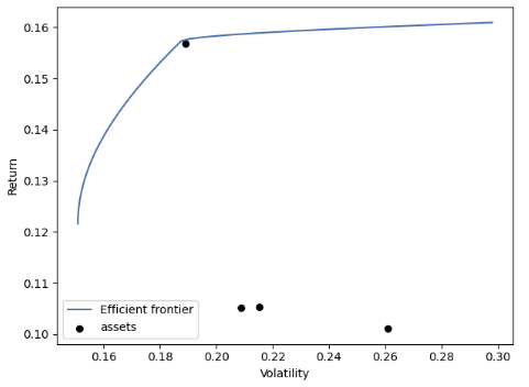
Read More:
Scenario 4: PyPortfolioOpt Risk Models & IPO
Stocks: Well-Diversified Portfolios of 15 and 20 Assets
portfolio1=['GOOG', 'AAPL', 'FB', 'BABA', 'AMZN', 'GE', 'AMD', 'WMT', 'BAC', 'GM',
       'T', 'UAA', 'SHLD', 'XOM', 'RRC', 'BBY', 'MA', 'PFE', 'JPM', 'SBUX']

portfolio2 = ["MSFT", "AMZN", "KO", "MA", "COST",
           "LUV", "XOM", "PFE", "JPM", "UNH",
           "ACN", "DIS", "GILD", "F", "TSLA"]
Time Horizons: 1989–2018 (portfolio 1) & 2014–2023 (portfolio 2)
Methods: Covariance-Based Risk Models & Available IPO Algorithms, viz.
CLA, dirichlet, EfficientFrontier, EfficientCVaR, sector constraints, L2 objective function, efficient risk, Discrete Allocation, Covariance Shrinkage, Efficient Semivariance
Objectives: Predicting Future Variance, mean/EMA historical and CAPM returns
Libraries: PyPortfolioOpt Cookbook
Read More:
Portfolio 1
- Importing libraries and preparing input stock data (portfolio 1) for IPO
import pandas as pd
import numpy as np
import matplotlib.pyplot as plt
import pypfopt
from pypfopt import risk_models, expected_returns, plotting
pypfopt.__version__
'1.5.3'

#Portfolio 1
df = pd.read_csv("stock_prices.csv", parse_dates=True, index_col="date")
past_df, future_df = df.iloc[:-250], df.iloc[-250:]- Applying the sample_cov risk model to the past and future DataFrames
future_cov = risk_models.sample_cov(future_df)

sample_cov = risk_models.sample_cov(past_df)
plotting.plot_covariance(sample_cov, plot_correlation=True)
plotting.plot_covariance(future_cov, plot_correlation=True)
plt.show()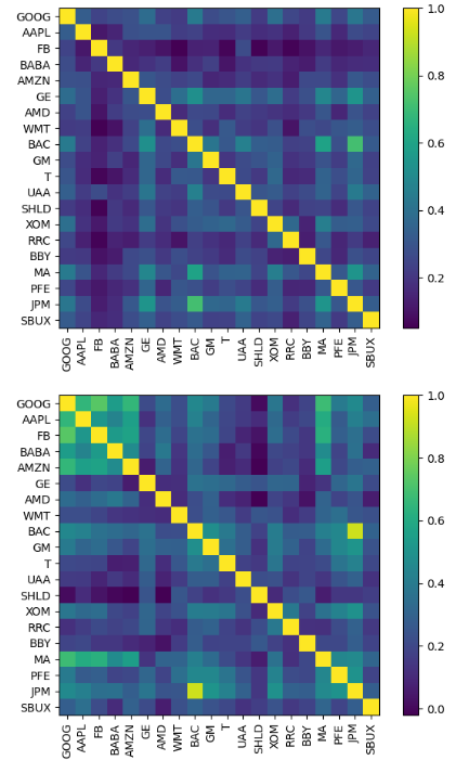
- Comparing MAE of different risk models
future_variance = np.diag(future_cov)
mean_abs_errors = []

risk_methods = [
    "sample_cov",
    "semicovariance",
    "exp_cov",
    "ledoit_wolf",
    "ledoit_wolf_constant_variance",
    "ledoit_wolf_single_factor",
    "ledoit_wolf_constant_correlation",
    "oracle_approximating",
]

for method in risk_methods:
    S = risk_models.risk_matrix(df, method=method)
    variance = np.diag(S)
    mean_abs_errors.append(np.sum(np.abs(variance - future_variance)) / len(variance))

xrange = range(len(mean_abs_errors))
plt.barh(xrange, mean_abs_errors)
plt.yticks(xrange, risk_methods)
plt.show()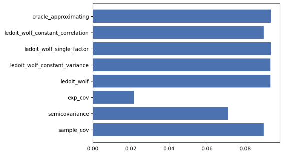
- Applying the exp_cov risk model to the past and future DataFrames
exp_cov = risk_models.exp_cov(past_df)
plotting.plot_covariance(exp_cov, plot_correlation=True)
plotting.plot_covariance(future_cov, plot_correlation=True)
plt.show()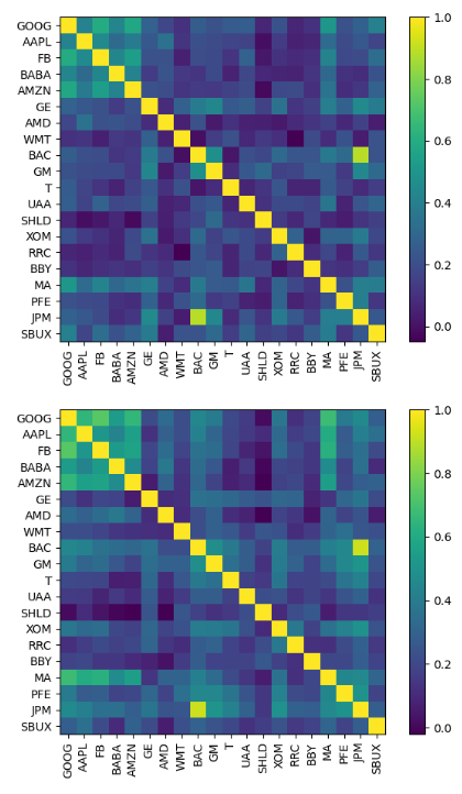
- Comparing MAE of different expected returns applied to the future DataFrame
future_rets = expected_returns.mean_historical_return(future_df)
mean_abs_errors = []
return_methods = [
    "mean_historical_return",
    "ema_historical_return",
    "capm_return",
    ]

for method in return_methods:
    mu = expected_returns.return_model(past_df, method=method)
    mean_abs_errors.append(np.sum(np.abs(mu - future_rets)) / len(mu))

xrange = range(len(mean_abs_errors))
plt.barh(xrange, mean_abs_errors)
plt.yticks(xrange, return_methods)
plt.show()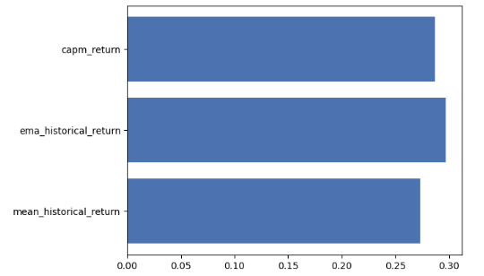
print(mean_abs_errors)
[0.2732675295106071, 0.29740354389638524, 0.28701847303235856]- Comparing the mean/ema historical return and CAPM returns for each individual stock
fig, axs = plt.subplots( 1, len(return_methods),sharey=True, figsize=(15,10))

for i, method in enumerate(return_methods):
    mu = expected_returns.return_model(past_df, method=method)
    axs[i].set_title(method)
    mu.plot.barh(ax=axs[i])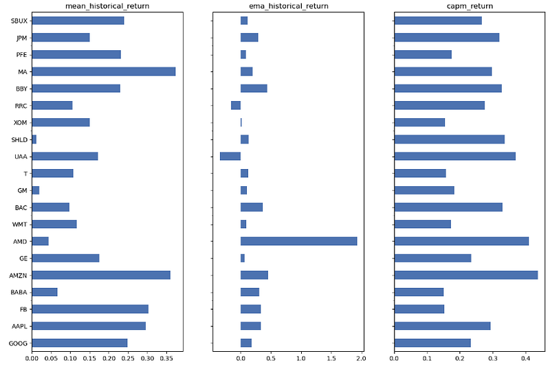
Portfolio 2
- Importing libraries and loading input stock data
import yfinance as yf
import matplotlib.pyplot as plt
import pandas as pd
import numpy as np
tickers = ["MSFT", "AMZN", "KO", "MA", "COST",
           "LUV", "XOM", "PFE", "JPM", "UNH",
           "ACN", "DIS", "GILD", "F", "TSLA"]
ohlc = yf.download(tickers, period="max")

prices = ohlc["Adj Close"].dropna(how="all")
prices.tail()
           ACN        AMZN        COST       DIS       F     GILD      JPM         KO        LUV        MA        MSFT       PFE      TSLA       UNH         XOM
Date
2023-03-31 285.809998 103.290001 496.869995 100.129997 12.60 82.970001 129.295288 62.029999 32.540001 362.840790 288.299988 40.799999 207.460007 472.589996 109.660004
2023-04-03 285.839996 102.410004 497.029999 99.760002 12.68 83.239998 129.146454 62.400002 31.690001 365.895966 287.230011 41.349998 194.770004 494.190002 116.129997
2023-04-04 285.839996 103.949997 497.730011 99.570000 12.72 82.120003 127.419998 62.209999 31.719999 363.329987 287.179993 40.900002 192.580002 493.250000 115.019997
2023-04-05 281.329987 101.099998 497.130005 99.910004 12.43 83.650002 127.610001 62.799999 31.580000 363.790009 284.339996 41.549999 185.520004 509.230011 116.989998
2023-04-06 281.700012 102.059998 485.980011 99.970001 12.33 83.370003 127.470001 62.840000 31.590000 361.470001 291.600006 41.500000 185.059998 512.809998 115.050003- Plotting stock prices
prices[prices.index >= "2014-01-01"].plot(figsize=(15,10));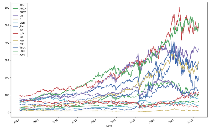
- Applying the risk_models.sample_cov model to these prices
from pypfopt import risk_models
from pypfopt import plotting

sample_cov = risk_models.sample_cov(prices, frequency=252)
sample_cov

      ACN     AMZN     COST      DIS      F       GILD     JPM       KO       LUV      MA       MSFT      PFE     TSLA     UNH      XOM
ACN 0.091047 0.047368 0.028694 0.041800 0.044966 0.028891 0.048398 0.020706 0.037365 0.046675 0.042606 0.025994 0.044706 0.030261 0.030249
AMZN 0.047368 0.328223 0.048238 0.056593 0.054212 0.057143 0.065805 0.020285 0.048216 0.057188 0.073389 0.031130 0.067031 0.034342 0.026733
COST 0.028694 0.048238 0.100966 0.032023 0.031947 0.026906 0.038356 0.021385 0.031193 0.032501 0.037554 0.025261 0.029679 0.027355 0.020312
DIS 0.041800 0.056593 0.032023 0.099784 0.041566 0.032046 0.047258 0.026103 0.039905 0.050994 0.043187 0.029207 0.044257 0.031657 0.025691
F 0.044966 0.054212 0.031947 0.041566 0.127992 0.030105 0.054766 0.026286 0.047190 0.062689 0.042048 0.027026 0.059955 0.029009 0.028220
GILD 0.028891 0.057143 0.026906 0.032046 0.030105 0.230470 0.042154 0.016764 0.030781 0.032162 0.034975 0.032445 0.031617 0.033702 0.021003
JPM 0.048398 0.065805 0.038356 0.047258 0.054766 0.042154 0.127442 0.027653 0.049041 0.068555 0.049036 0.032597 0.041645 0.038364 0.033168
KO 0.020706 0.020285 0.021385 0.026103 0.026286 0.016764 0.027653 0.053362 0.022847 0.026121 0.027759 0.025953 0.018689 0.022953 0.020577
LUV 0.037365 0.048216 0.031193 0.039905 0.047190 0.030781 0.049041 0.022847 0.138311 0.048528 0.036969 0.025762 0.043051 0.032155 0.023438
MA 0.046675 0.057188 0.032501 0.050994 0.062689 0.032162 0.068555 0.026121 0.048528 0.116744 0.049793 0.031913 0.049745 0.042009 0.041492
MSFT 0.042606 0.073389 0.037554 0.043187 0.042048 0.034975 0.049036 0.027759 0.036969 0.049793 0.114527 0.030579 0.053099 0.033850 0.028928
PFE 0.025994 0.031130 0.025261 0.029207 0.027026 0.032445 0.032597 0.025953 0.025762 0.031913 0.030579 0.075916 0.017928 0.028178 0.022933
TSLA 0.044706 0.067031 0.029679 0.044257 0.059955 0.031617 0.041645 0.018689 0.043051 0.049745 0.053099 0.017928 0.329399 0.030690 0.029405
UNH 0.030261 0.034342 0.027355 0.031657 0.029009 0.033702 0.038364 0.022953 0.032155 0.042009 0.033850 0.028178 0.030690 0.160524 0.022458
XOM 0.030249 0.026733 0.020312 0.025691 0.028220 0.021003 0.033168 0.020577 0.023438 0.041492 0.028928 0.022933 0.029405 0.022458 0.052893- Plotting the sample covariance matrix
plotting.plot_covariance(sample_cov, plot_correlation=True);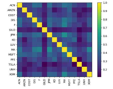
- Applying the isk_models.CovarianceShrinkage model to the stock prices
S = risk_models.CovarianceShrinkage(prices).ledoit_wolf()
plotting.plot_covariance(S, plot_correlation=True);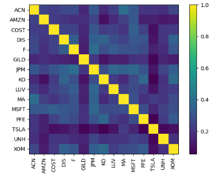
- Computing CAPM expected returns of portfolio 2
from pypfopt import expected_returns

mu = expected_returns.capm_return(prices)
mu

ACN     0.208064
AMZN    0.349090
COST    0.190865
DIS     0.219967
F       0.222607
GILD    0.244659
JPM     0.245611
KO      0.144716
LUV     0.223131
MA      0.255686
MSFT    0.234936
PFE     0.173457
TSLA    0.294081
UNH     0.213354
XOM     0.138895
Name: mkt, dtype: float64

mu.plot.barh(figsize=(10,6));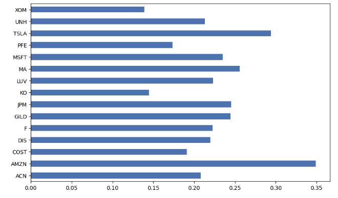
- Applying the EfficientFrontier IPO method with the Covariance Shrinkage risk model to portfolio 2
from pypfopt import EfficientFrontier
S = risk_models.CovarianceShrinkage(prices).ledoit_wolf()

# You don't have to provide expected returns in this case
ef = EfficientFrontier(None, S, weight_bounds=(None, None))
ef.min_volatility()
weights = ef.clean_weights()
weights
OrderedDict([('ACN', 0.22843),
             ('AMZN', 0.00616),
             ('COST', 0.09999),
             ('DIS', -0.02036),
             ('F', -0.02273),
             ('GILD', 0.04898),
             ('JPM', -0.04691),
             ('KO', 0.13455),
             ('LUV', 0.02459),
             ('MA', 0.23496),
             ('MSFT', -0.00235),
             ('PFE', 0.07144),
             ('TSLA', 0.12347),
             ('UNH', 0.0355),
             ('XOM', 0.08427)])

pd.Series(weights).plot.barh();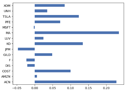
- Portfolio 2 performance
ef.portfolio_performance(verbose=True);
Annual volatility: 12.2%- Applying Discrete Allocation to portfolio 2
from pypfopt import DiscreteAllocation

latest_prices = prices.iloc[-1]  # prices as of the day you are allocating
da = DiscreteAllocation(weights, latest_prices, total_portfolio_value=20000, short_ratio=0.3)
alloc, leftover = da.lp_portfolio()
print(f"Discrete allocation performed with ${leftover:.2f} leftover")
alloc
Discrete allocation performed with $58.92 leftover
{'ACN': 15,
 'AMZN': 1,
 'COST': 4,
 'GILD': 11,
 'KO': 39,
 'LUV': 14,
 'MA': 12,
 'PFE': 32,
 'TSLA': 12,
 'UNH': 1,
 'XOM': 13,
 'F': -178,
 'JPM': -25,
'MSFT': -2}- Performing sector mapping to include group industry constraints
sector_mapper = {
    "MSFT": "Tech",
    "AMZN": "Consumer Discretionary",
    "KO": "Consumer Staples",
    "MA": "Financial Services",
    "COST": "Consumer Staples",
    "LUV": "Aerospace",
    "XOM": "Energy",
    "PFE": "Healthcare",
    "JPM": "Financial Services",
    "UNH": "Healthcare",
    "ACN": "Misc",
    "DIS": "Media",
    "GILD": "Healthcare",
    "F": "Auto",
    "TSLA": "Auto"
}

sector_lower = {
    "Consumer Staples": 0.1, # at least 10% to staples
    "Tech": 0.05 # at least 5% to tech
    # For all other sectors, it will be assumed there is no lower bound
}

sector_upper = {
    "Tech": 0.2,
    "Aerospace":0.1,
    "Energy": 0.1,
    "Auto":0.15
}- Optimizing portfolio weights by adding constraints
mu = expected_returns.capm_return(prices)
S = risk_models.CovarianceShrinkage(prices).ledoit_wolf()

ef = EfficientFrontier(mu, S)  # weight_bounds automatically set to (0, 1)
ef.add_sector_constraints(sector_mapper, sector_lower, sector_upper)

amzn_index = ef.tickers.index("AMZN")
ef.add_constraint(lambda w: w[amzn_index] == 0.10)

tsla_index = ef.tickers.index("TSLA")
ef.add_constraint(lambda w: w[tsla_index] <= 0.05)

ef.add_constraint(lambda w: w[10] >= 0.05)

ef.max_sharpe()
weights = ef.clean_weights()- Plotting the ordered dictionary of optimized weights
weights

OrderedDict([('ACN', 0.16879),
             ('AMZN', 0.1),
             ('COST', 0.05458),
             ('DIS', 0.0),
             ('F', 0.0),
             ('GILD', 0.06404),
             ('JPM', 0.0),
             ('KO', 0.04542),
             ('LUV', 0.02193),
             ('MA', 0.3823),
             ('MSFT', 0.05),
             ('PFE', 0.02692),
             ('TSLA', 0.05),
             ('UNH', 0.03601),
             ('XOM', 0.0)])

pd.Series(weights).plot.pie(figsize=(10,10));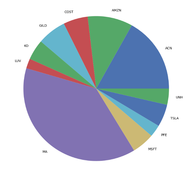
- Defining the optimal weight constraint per sector
for sector in set(sector_mapper.values()):
    total_weight = 0
    for t,w in weights.items():
        if sector_mapper[t] == sector:
            total_weight += w
    print(f"{sector}: {total_weight:.3f}")

Financial Services: 0.382
Consumer Staples: 0.100
Aerospace: 0.022
Auto: 0.050
Misc: 0.169
Consumer Discretionary: 0.100
Media: 0.000
Healthcare: 0.127
Tech: 0.050
Energy: 0.000- Running EfficientFrontier IPO with sector constraints and efficient_risk
ef = EfficientFrontier(mu, S)
ef.add_sector_constraints(sector_mapper, sector_lower, sector_upper)
ef.efficient_risk(target_volatility=0.15)
weights = ef.clean_weights()
weights

OrderedDict([('ACN', 0.00967),
             ('AMZN', 0.16383),
             ('COST', 0.09374),
             ('DIS', 0.0),
             ('F', 0.0),
             ('GILD', 0.06523),
             ('JPM', 0.0),
             ('KO', 0.00626),
             ('LUV', 0.00466),
             ('MA', 0.444),
             ('MSFT', 0.05),
             ('PFE', 0.0),
             ('TSLA', 0.15),
             ('UNH', 0.01261),
('XOM', 0.0)])- Counting stocks with zero weights
num_small = len([k for k in weights if weights[k] <= 1e-4])
print(f"{num_small}/{len(ef.tickers)} tickers have zero weight")
5/15 tickers have zero weight- Examining the portfolio performance
ef.portfolio_performance(verbose=True);
Expected annual return: 26.7%
Annual volatility: 15.0%
Sharpe Ratio: 1.65- Adding the L2 regularization objective function with the tuning parameter gamma=0.1
from pypfopt import objective_functions

# You must always create a new efficient frontier object
ef = EfficientFrontier(mu, S)
ef.add_sector_constraints(sector_mapper, sector_lower, sector_upper)
ef.add_objective(objective_functions.L2_reg, gamma=0.1)  # gamma is the tuning parameter
ef.efficient_risk(0.15)
weights = ef.clean_weights()
weights
OrderedDict([('ACN', 0.06921),
             ('AMZN', 0.18629),
             ('COST', 0.08355),
             ('DIS', 0.01489),
             ('F', 0.0),
             ('GILD', 0.07874),
             ('JPM', 0.04271),
             ('KO', 0.01645),
             ('LUV', 0.03281),
             ('MA', 0.23867),
             ('MSFT', 0.05),
             ('PFE', 0.0),
             ('TSLA', 0.15),
             ('UNH', 0.03668),
             ('XOM', 0.0)])
- Counting the zero-weight tickers
num_small = len([k for k in weights if weights[k] <= 1e-4])
print(f"{num_small}/{len(ef.tickers)} tickers have zero weight")
3/15 tickers have zero weight- Running EfficientFrontier by adding constraints, the efficient risk model, and L2 regularization with the tuning parameter gamma=1.0
ef = EfficientFrontier(mu, S)
ef.add_sector_constraints(sector_mapper, sector_lower, sector_upper)
ef.add_objective(objective_functions.L2_reg, gamma=1)  # gamma is the tuning parameter
ef.efficient_risk(0.15)
weights = ef.clean_weights()
weights

OrderedDict([('ACN', 0.05956),
             ('AMZN', 0.12684),
             ('COST', 0.06125),
             ('DIS', 0.06355),
             ('F', 0.05615),
             ('GILD', 0.07647),
             ('JPM', 0.07598),
             ('KO', 0.03875),
             ('LUV', 0.0654),
             ('MA', 0.08332),
             ('MSFT', 0.07136),
             ('PFE', 0.04172),
             ('TSLA', 0.09385),
             ('UNH', 0.06112),
             ('XOM', 0.02469)])

pd.Series(weights).plot.pie(figsize=(10, 10));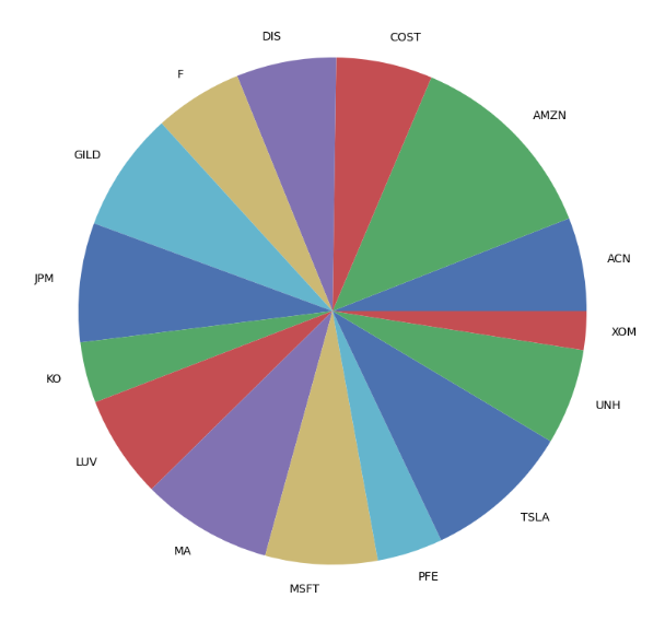
- Portfolio performance summary
ef.portfolio_performance(verbose=True);
Expected annual return: 24.2%
Annual volatility: 15.0%
Sharpe Ratio: 1.48- Running EfficientFrontier without weights bounds by adding the L2 regularization and the market-neutral efficient return with target_return=0.07
ef = EfficientFrontier(mu, S, weight_bounds=(None, None))
ef.add_objective(objective_functions.L2_reg)
ef.efficient_return(target_return=0.07, market_neutral=True)
weights = ef.clean_weights()
weights

OrderedDict([('ACN', -0.03031),
             ('AMZN', 0.21164),
             ('COST', -0.05977),
             ('DIS', -0.00357),
             ('F', -0.00038),
             ('GILD', 0.03495),
             ('JPM', 0.04047),
             ('KO', -0.13985),
             ('LUV', -0.00028),
             ('MA', 0.0588),
             ('MSFT', 0.01942),
             ('PFE', -0.08738),
             ('TSLA', 0.12484),
             ('UNH', -0.01647),
('XOM', -0.15212)])- Portfolio performance summary
ef.portfolio_performance(verbose=True);
Expected annual return: 7.0%
Annual volatility: 10.6%
Sharpe Ratio: 0.47- Plotting the optimized weights and the semicovariance matrix
pd.Series(weights).plot.barh(figsize=(10,6));

print(f"Net weight: {sum(weights.values()):.2f}")
Net weight: -0.00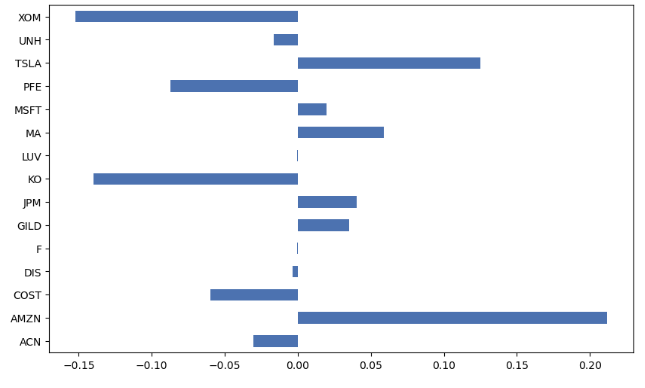
semicov = risk_models.semicovariance(prices, benchmark=0)
plotting.plot_covariance(semicov);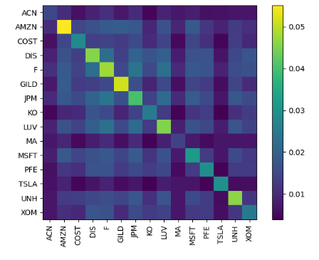
- Running EfficientFrontier with semicov
ef = EfficientFrontier(mu, semicov)
ef.efficient_return(0.2)
weights = ef.clean_weights()
weights

OrderedDict([('ACN', 0.25277),
             ('AMZN', 0.0),
             ('COST', 0.08549),
             ('DIS', 0.0),
             ('F', 0.0),
             ('GILD', 0.01648),
             ('JPM', 0.0),
             ('KO', 0.14564),
             ('LUV', 0.0),
             ('MA', 0.31895),
             ('MSFT', 0.0),
             ('PFE', 0.05079),
             ('TSLA', 0.11332),
             ('UNH', 0.00218),
('XOM', 0.01438)])- Portfolio performance summary
ef.portfolio_performance(verbose=True);
Expected annual return: 22.0%
Annual volatility: 9.3%
Sharpe Ratio: 2.16
- Running EfficientSemivariance with expected returns while checking the portfolio performance
returns = expected_returns.returns_from_prices(prices)
returns = returns.dropna()
from pypfopt import EfficientSemivariance

es = EfficientSemivariance(mu, returns)
es.efficient_return(0.2)
es.portfolio_performance(verbose=True);
Expected annual return: 20.0%
Annual semi-deviation: 10.7%
Sortino Ratio: 1.69

es.weights = ef.weights
es.portfolio_performance(verbose=True);
xpected annual return: 22.0%
Annual semi-deviation: 14.0%
Sortino Ratio: 1.43- Printing expected returns per stock
returns = expected_returns.returns_from_prices(prices).dropna()
returns.head()
ACN AMZN COST DIS F GILD JPM KO LUV MA MSFT PFE TSLA UNH XOM
Date
2010-06-30 0.000000 0.005985 -0.014381 -0.024768 0.020243 -0.019731 -0.012143 -0.004172 0.000000 -0.017045 -0.012870 -0.001401 -0.002511 -0.008034 -0.003840
2010-07-01 -0.009573 0.015559 0.001277 -0.000317 0.048611 -0.004084 -0.013129 -0.001796 -0.010801 0.016652 0.006519 -0.002104 -0.078473 -0.019366 -0.008060
2010-07-02 -0.008882 -0.016402 -0.012205 -0.003493 -0.027436 0.021383 -0.006929 0.000400 -0.021838 0.000345 0.004749 -0.006325 -0.125683 0.016158 -0.000706
2010-07-06 0.012388 0.008430 -0.004241 0.010835 -0.011673 -0.002868 0.013955 0.007592 -0.011163 -0.013513 0.023636 0.010608 -0.160937 0.020848 0.015732
2010-07-07 0.022130 0.030620 0.005370 0.044767 0.042323 0.004889 0.050096 0.020623 0.062089 0.037694 0.020151 0.023093 -0.019243 0.010730 0.016881- Running EfficientFrontier with max Sharpe ratio while examining the portfolio performance
ef = EfficientFrontier(mu, S)
ef.max_sharpe()
weight_arr = ef.weights
ef.portfolio_performance(verbose=True);
Expected annual return: 25.1%
Annual volatility: 13.4%
Sharpe Ratio: 1.73- Plotting the portfolio returns histogram
portfolio_rets = (returns * weight_arr).sum(axis=1)
portfolio_rets.hist(bins=50);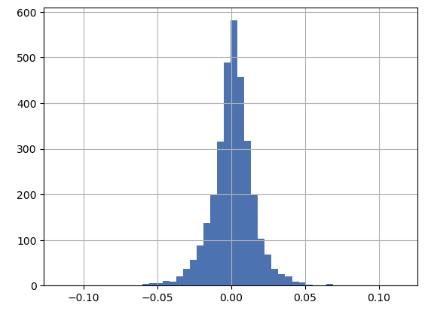
- Comparing VaR and CVaR
var = portfolio_rets.quantile(0.05)
cvar = portfolio_rets[portfolio_rets <= var].mean()
print("VaR: {:.2f}%".format(100*var))
print("CVaR: {:.2f}%".format(100*cvar))

VaR: -2.26%
CVaR: -3.35%- Running EfficientCVaR with the performance summary
from pypfopt import EfficientCVaR

ec = EfficientCVaR(mu, returns)
ec.efficient_risk(target_cvar=0.025)
ec.portfolio_performance(verbose=True);

Expected annual return: 23.2%
Conditional Value at Risk: 2.50%- Running the Critical Line Algorithm
from pypfopt import CLA, plotting

cla = CLA(mu, S)
cla.max_sharpe()
cla.portfolio_performance(verbose=True);
from pypfopt import CLA, plotting

cla = CLA(mu, S)
cla.max_sharpe()
cla.portfolio_performance(verbose=True);
Expected annual return: 24.8%
Annual volatility: 13.2%
Sharpe Ratio: 1.73
ax = plotting.plot_efficient_frontier(cla, showfig=False)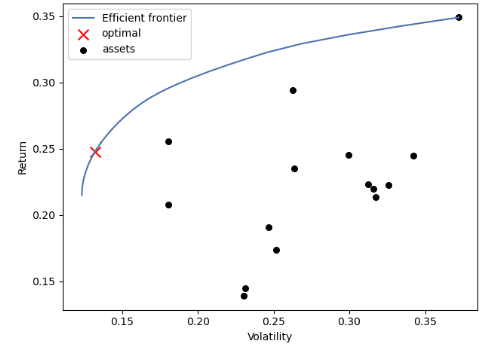
- Running Efficient Frontier with random portfolios (Monte Carlo)
n_samples = 10000
w = np.random.dirichlet(np.ones(len(mu)), n_samples)
rets = w.dot(mu)
stds = np.sqrt((w.T * (S @ w.T)).sum(axis=0))
sharpes = rets / stds

print("Sample portfolio returns:", rets)
print("Sample portfolio volatilities:", stds)
Sample portfolio returns: [0.23104048 0.24957187 0.22126853 ... 0.22765487 0.21850872 0.23138569]
Sample portfolio volatilities: 0       0.159978
1       0.163969
2       0.146534
3       0.158051
4       0.147951
          ...
9995    0.145396
9996    0.146341
9997    0.168378
9998    0.193611
9999    0.152335
Length: 10000, dtype: float64
# Plot efficient frontier with Monte Carlo sim
ef = EfficientFrontier(mu, S)
fig, ax = plt.subplots()
plotting.plot_efficient_frontier(ef, ax=ax, show_assets=False)
# Find and plot the tangency portfolio
ef2 = EfficientFrontier(mu, S)
ef2.max_sharpe()
ret_tangent, std_tangent, _ = ef2.portfolio_performance()
# Plot random portfolios
ax.scatter(stds, rets, marker=".", c=sharpes, cmap="viridis_r")
# Format
ax.set_title("Efficient Frontier with random portfolios")
ax.legend()
plt.tight_layout()
plt.show()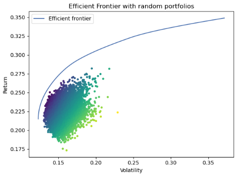
def plot_efficient_frontier_and_max_sharpe(mu, S):
    # Optimize portfolio for maximal Sharpe ratio
    ef = EfficientFrontier(mu, S)

    fig, ax = plt.subplots(figsize=(8,6))
    ef_max_sharpe = copy.deepcopy(ef)
    plotting.plot_efficient_frontier(ef, ax=ax, show_assets=False)

    # Find the max sharpe portfolio
    ef_max_sharpe.max_sharpe(risk_free_rate=0.02)
    ret_tangent, std_tangent, _ = ef_max_sharpe.portfolio_performance()
    ax.scatter(std_tangent, ret_tangent, marker="*", s=100, c="r", label="Max Sharpe")

    # Generate random portfolios
    n_samples = 1000
    w = np.random.dirichlet(np.ones(ef.n_assets), n_samples)
    rets = w.dot(ef.expected_returns)
    stds = np.sqrt(np.diag(w @ ef.cov_matrix @ w.T))
    sharpes = rets / stds
    ax.scatter(stds, rets, marker=".", c=sharpes, cmap="viridis_r")

    # Output
    ax.set_title("Efficient Frontier with Random Portfolios")
    ax.legend()
    plt.tight_layout()
    plt.show()

plot_efficient_frontier_and_max_sharpe(mu, S)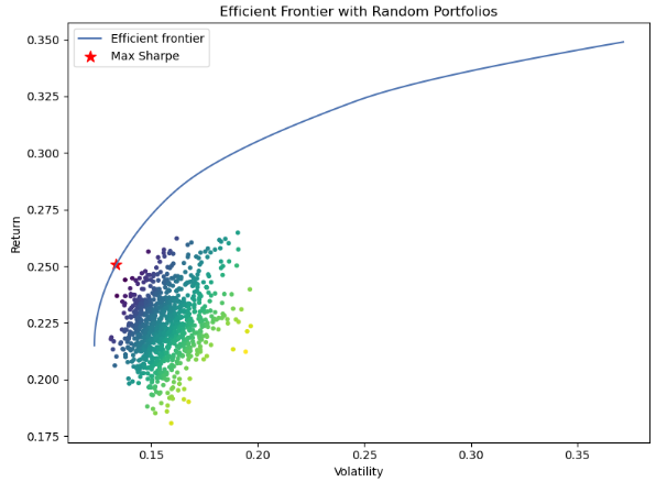
Scenario 5: Mean-Variance MPT
Stocks: Well-diversified portfolio of 6 assets
stocks = ['MA', 'WM', 'AZN', 'SBUX', 'CLX', 'XOM']Time Horizon: start=”2013–01–01", end=”2023–04–06"
Methods: Monte Carlo Efficient Frontier
Objectives: max Sharpe ratio
Libraries: yfinance, PyPortfolioOpt
- Importing libraries and reading input stock data
from pypfopt.discrete_allocation import DiscreteAllocation, get_latest_prices
from pypfopt import EfficientFrontier
from pypfopt import risk_models
from pypfopt import expected_returns
from pypfopt import plotting
import copy
import numpy as np
import pandas as pd
import plotly.express as px
import matplotlib.pyplot as plt
import seaborn as sns
from pandas_datareader import data as pdr
import pandas_datareader.data as web
import datetime as dt

import yfinance as yf
stocks_df = yf.download("MA WM AZN SBUX CLX XOM", start="2013-01-01", end="2023-04-06")['Adj Close']
stocks_df.tail()

           AZN       CLX        MA         SBUX       WM         XOM
Date
2023-03-30 69.199997 154.440002 358.697296 101.320000 161.529999 109.489998
2023-03-31 69.410004 158.240005 362.840790 104.129997 163.169998 109.660004
2023-04-03 69.910004 156.750000 365.895966 104.849998 163.869995 116.129997
2023-04-04 70.250000 155.899994 363.329987 104.000000 163.529999 115.019997
2023-04-05 72.050003 157.419998 363.790009 104.900002 162.820007 116.989998- Plotting the Adj Close price of individual stocks with Plotly
fig_price = px.line(stocks_df, title='Price of Individual Stocks')
fig_price.show()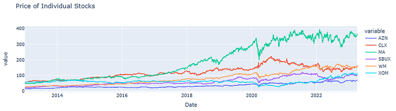
- Calculating and plotting daily returns of individual stocks
daily_returns = stocks_df.pct_change().dropna()
daily_returns.tail()
           AZN       CLX       MA       SBUX     WM        XOM
Date
2023-03-30 0.008158 -0.006817 -0.000751 0.006957 0.028591 0.004864
2023-03-31 0.003035 0.024605 0.011552 0.027734 0.010153 0.001553
2023-04-03 0.007204 -0.009416 0.008420 0.006914 0.004290 0.059000
2023-04-04 0.004863 -0.005423 -0.007013 -0.008107 -0.002075 -0.009558
2023-04-05 0.025623 0.009750 0.001266 0.008654 -0.004342 0.017127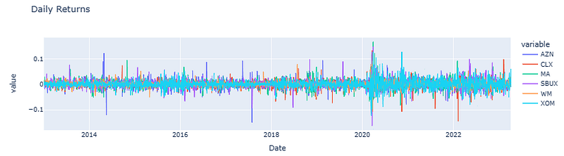
- Calculating std of daily returns
daily_returns.std()
AZN     0.015491
CLX     0.013763
MA      0.017123
SBUX    0.016214
WM      0.011630
XOM     0.016923
dtype: float64
- Examining the seaborn distribution plot of daily returns
sns.displot(data=daily_returns[['AZN', 'CLX','MA','SBUX','WM','XOM']], kind = 'kde', aspect = 2.5)
plt.xlim(-0.1, 0.1)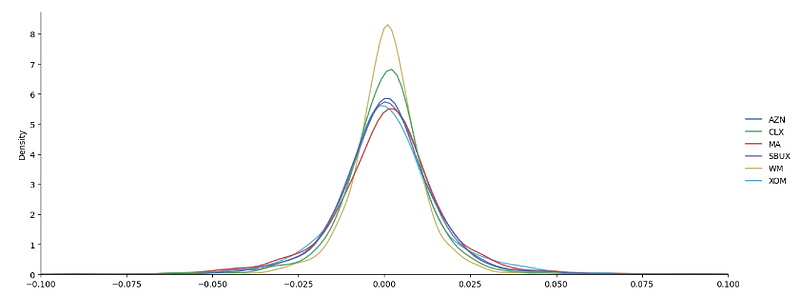
- Plotting the Cumulative Returns of Individual Stocks Starting with $100
def plot_cum_returns(data, title):
    daily_cum_returns = (1 + daily_returns).cumprod()*100
    fig = px.line(daily_cum_returns, title=title)
    return fig

fig_cum_returns = plot_cum_returns(stocks_df, 'Cumulative Returns of Individual Stocks Starting with $100')
fig_cum_returns.show()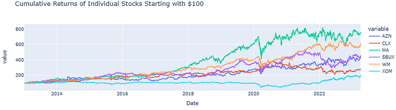
- Plotting the stock correlation matrix
corr_df = stocks_df.corr().round(2) # round to 2 decimal places
fig_corr = px.imshow(corr_df, text_auto=True, title = 'Correlation between Stocks')
fig_corr.show()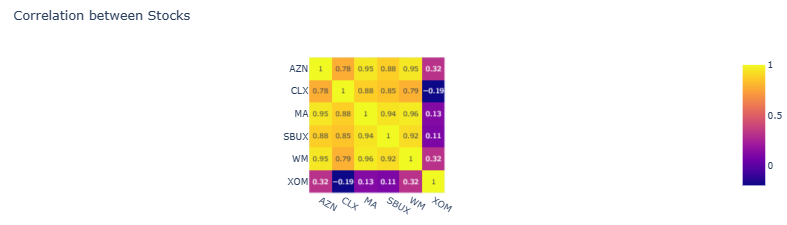
- Calculating expected returns and sample covariance matrix
# Calculate expected returns and sample covariance matrix
mu = expected_returns.mean_historical_return(stocks_df)
S = risk_models.sample_cov(stocks_df)

print(mu)

AZN     0.156955
CLX     0.106144
MA      0.218699
SBUX    0.159896
WM      0.193191
XOM     0.071530
dtype: float64- Plotting the MPT efficient frontier with random portfolios vs max Sharpe ratio
def plot_efficient_frontier_and_max_sharpe(mu, S):
    # Optimize portfolio for maximal Sharpe ratio
    ef = EfficientFrontier(mu, S)

    fig, ax = plt.subplots(figsize=(8,6))
    ef_max_sharpe = copy.deepcopy(ef)
    plotting.plot_efficient_frontier(ef, ax=ax, show_assets=False)

    # Find the max sharpe portfolio
    ef_max_sharpe.max_sharpe(risk_free_rate=0.02)
    ret_tangent, std_tangent, _ = ef_max_sharpe.portfolio_performance()
    ax.scatter(std_tangent, ret_tangent, marker="*", s=100, c="r", label="Max Sharpe")

    # Generate random portfolios
    n_samples = 1000
    w = np.random.dirichlet(np.ones(ef.n_assets), n_samples)
    rets = w.dot(ef.expected_returns)
    stds = np.sqrt(np.diag(w @ ef.cov_matrix @ w.T))
    sharpes = rets / stds
    ax.scatter(stds, rets, marker=".", c=sharpes, cmap="viridis_r")

    # Output
    ax.set_title("Efficient Frontier with Random Portfolios")
    ax.legend()
    plt.tight_layout()
    plt.show()

plot_efficient_frontier_and_max_sharpe(mu, S)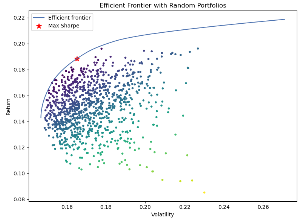
- Calculating the optimized portfolio weights
ef = EfficientFrontier(mu, S)
ef.max_sharpe(risk_free_rate=0.02)
weights = ef.clean_weights()
print(weights)
OrderedDict([('AZN', 0.15466), ('CLX', 0.04592), ('MA', 0.18582), ('SBUX', 0.0), ('WM', 0.61359), ('XOM', 0.0)])

weights_df = pd.DataFrame.from_dict(weights, orient = 'index')
weights_df.columns = ['weights']
weights_df

     weights
AZN  0.15466
CLX  0.04592
MA   0.18582
SBUX 0.00000
WM   0.61359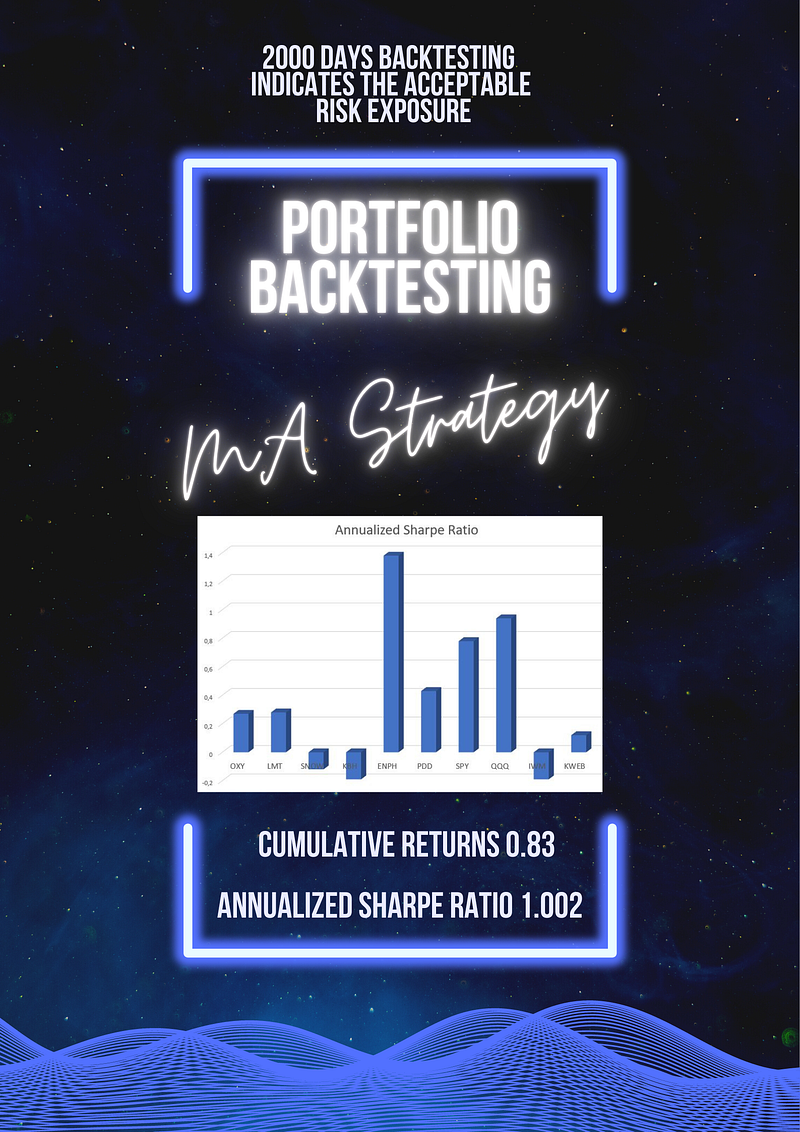
XOM 0.00000- Calculating the Expected annual return, Annual volatility, the Sharpe ratio, and the Optimized Portfolio
expected_annual_return, annual_volatility, sharpe_ratio = ef.portfolio_performance()

print('Expected annual return: {}%'.format((expected_annual_return*100).round(2)))
print('Annual volatility: {}%'.format((annual_volatility*100).round(2)))
print('Sharpe ratio: {}'.format(sharpe_ratio.round(2)))

Expected annual return: 18.83%
Annual volatility: 16.51%
Sharpe ratio: 1.02

stocks_df['Optimized Portfolio'] = 0

for ticker, weight in weights.items():
    stocks_df['Optimized Portfolio'] += stocks_df[ticker]*weight

stocks_df.head()

           AZN      CLX        MA       SBUX      WM        XOM    Optimized Portfolio
Date
2013-01-02 16.17679 55.996990 47.946114 22.947464 26.652275 57.639828 30.336200
2013-01-03 16.14661 55.845818 48.014702 23.101843 26.746429 57.535881 30.395108
2013-01-04 16.14661 56.465561 48.012817 23.235355 26.738588 57.802296 30.418405
2013-01-07 16.13320 56.238838 48.844879 23.247875 26.652275 57.133026 30.507573
2013-01-08 16.14661 56.405109 48.684109 23.206150 26.707193 57.490395 30.521105- Plotting the Cumulative Returns of Optimized Portfolio Starting with $100
fig_cum_returns_optimized = plot_cum_returns(stocks_df['Optimized Portfolio'], 'Cumulative Returns of Optimized Portfolio Starting with $100')
fig_cum_returns_optimized.show()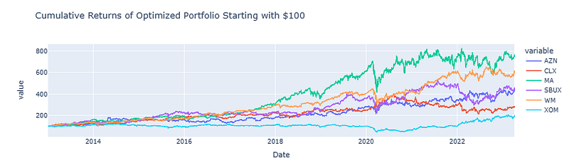
Read More
- Mean-Variance Optimization
- Max Sharpe Ratio Portfolio Optimization for Stocks Using PyPortfolioOpt.ipynb
Scenario 6: Black-Litterman (BL) & Covariance Shrinkage
Stocks: Well-diversified portfolio of 9 assets vs SPY ETF benchmark
tickers = ["XOM", "AZN", "CLX", "MA", "SBUX", "WM", "MO", "JPM", "COST"]Time Horizon: 1993–2023, period=”max”
Methods: the Black-Litterman Model
Objectives: Combining BL & Risk Models
Libraries: yfinance, PyPortfolioOpt
- Importing libraries and reading input stock data
import numpy as np
import pandas as pd
import matplotlib.pyplot as plt
import yfinance as yf
tickers = ["XOM", "AZN", "CLX", "MA", "SBUX", "WM", "MO", "JPM", "COST"]
ohlc = yf.download(tickers, period="max")
prices = ohlc["Adj Close"]
prices.tail()
           AZN       CLX        COST       JPM        MA         MO        SBUX       WM         XOM
Date
2023-03-31 69.410004 158.240005 496.869995 129.295288 362.840790 44.619999 104.129997 163.169998 109.660004
2023-04-03 69.910004 156.750000 497.029999 129.146454 365.895966 44.980000 104.849998 163.869995 116.129997
2023-04-04 70.250000 155.899994 497.730011 127.419998 363.329987 44.450001 104.000000 163.529999 115.019997
2023-04-05 72.050003 157.419998 497.130005 127.610001 363.790009 44.430000 104.900002 162.820007 116.989998
2023-04-06 72.339996 157.759995 485.980011 127.470001 361.470001 44.430000 104.680000 163.660004 115.050003- Comparing to the SPY ETF Adj Close price
market_prices = yf.download("SPY", period="max")["Adj Close"]
market_prices.head()
Date
1993-01-29    25.122337
1993-02-01    25.301022
1993-02-02    25.354639
1993-02-03    25.622641
1993-02-04    25.729851
Name: Adj Close, dtype: float64- Examining the market cap of individual stocks (cf. market capitalization-weighted portfolio)
mcaps = {}
import pandas_datareader as web
mcaps = web.get_quote_yahoo(tickers)['marketCap']
print(mcaps)
XOM     468366262272
AZN     225498234880
CLX      19487303680
MA      344568758272
SBUX    120308719616
WM       66571489280
MO       79358648320
JPM     373673230336
COST    215523885056
Name: marketCap, dtype: int64- Using the BL market implied risk aversion and the Covariance Shrinkage risk model
from pypfopt import black_litterman, risk_models
from pypfopt import BlackLittermanModel, plotting

S = risk_models.CovarianceShrinkage(prices).ledoit_wolf()
delta = black_litterman.market_implied_risk_aversion(market_prices)
delta
2.5290120773891447
- Plotting the stock correlation matrix
plotting.plot_covariance(S, plot_correlation=True);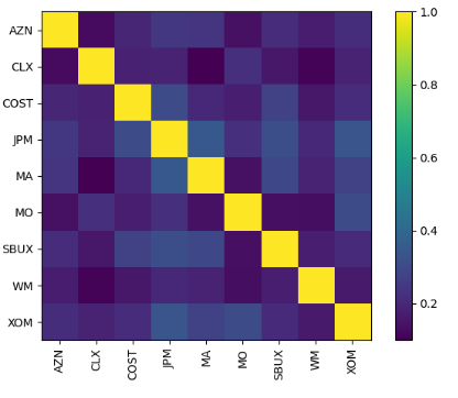
- Calculating the BL market implied prior returns
market_prior = black_litterman.market_implied_prior_returns(mcaps, delta, S)
market_prior
AZN     0.052048
CLX     0.047593
COST    0.068028
JPM     0.105222
MA      0.059766
MO      0.057295
SBUX    0.069242
WM      0.052832
XOM     0.080756
dtype: float64- Plotting the BL market implied prior returns
market_prior.plot.barh(figsize=(10,5));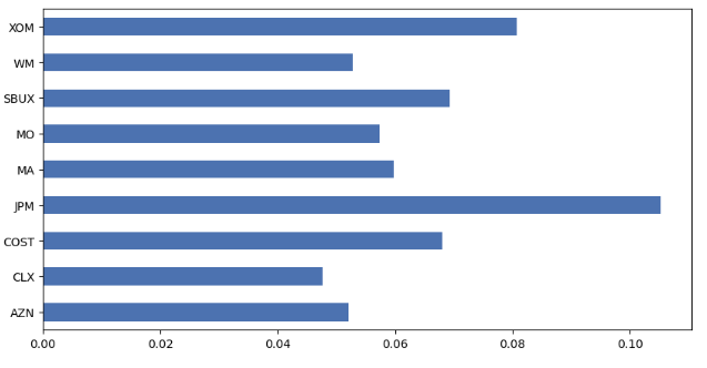
- Adding absolute views and view confidences options to the BL model
viewdict = {
    "AZN": 0.40,
    "CLX": 0.30,
    "MA": 0.7,
    "SBUX": 0.4,
    "WM": 0.6,
    "XOM": 0.2
}

bl = BlackLittermanModel(S, pi=market_prior, absolute_views=viewdict)

confidences = [
    0.1,
    0.1,
    0.2,
    0.1,
    0.2,
    0.3
]

bl = BlackLittermanModel(S, pi=market_prior, absolute_views=viewdict, omega="idzorek", view_confidences=confidences)- The BL model outputs posterior estimates of the returns and covariance matrix
np.diag(bl.omega)
array([0.01546742, 0.03113534, 0.00648636, 0.03241998, 0.01408768,
       0.00617762])

fig, ax = plt.subplots(figsize=(7,7))
im = ax.imshow(bl.omega)


ax.set_xticks(np.arange(len(bl.tickers)))
ax.set_yticks(np.arange(len(bl.tickers)))

ax.set_xticklabels(bl.tickers)
ax.set_yticklabels(bl.tickers)
plt.show()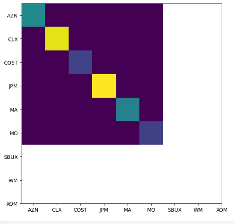
Scenario 7: Hierarchical Risk Parity
Stocks: Well-diversified portfolio of 15 assets
tickers = ["BLK", "BAC", "AAPL", "TM", "WMT",
           "JD", "INTU", "MA", "UL", "CVS",
           "DIS", "AMD", "NVDA", "PBI", "TGT"]
Time Horizon: 1993–2023, period=”max”
Methods: HRPOpt
Objectives: Portfolio Performance Analysis
Libraries: yfinance, PyPortfolioOpt
- Importing libraries and reading input stock data
import numpy as np
import pandas as pd
import matplotlib.pyplot as plt
import yfinance as yf
import pypfopt

pypfopt.__version__
'1.5.3'

tickers = ["BLK", "BAC", "AAPL", "TM", "WMT",
           "JD", "INTU", "MA", "UL", "CVS",
           "DIS", "AMD", "NVDA", "PBI", "TGT"]

ohlc = yf.download(tickers, period="max")
prices = ohlc["Adj Close"]
prices.tail()

           AAPL       AMD        BAC      BLK        CVS       DIS       INTU         JD        MA        NVDA       PBI    TGT       TM        UL         WMT
Date
2023-03-31 164.899994 98.010002 28.600000 669.119995 74.309998 100.129997 445.038116 43.239620 362.840790 277.769989 3.89 165.630005 141.690002 51.930000 147.449997
2023-04-03 166.169998 96.559998 28.590000 666.409973 76.089996 99.760002 439.887299 41.771702 365.895966 279.649994 3.83 166.059998 142.339996 52.700001 148.690002
2023-04-04 165.630005 95.870003 27.980000 659.109985 76.250000 99.570000 439.028839 41.220001 363.329987 274.529999 3.83 166.050003 142.139999 52.939999 147.229996
2023-04-05 163.759995 92.559998 27.639999 656.039978 77.750000 99.910004 438.369995 40.500000 363.790009 268.809998 3.67 165.240005 140.419998 53.320000 149.669998
2023-04-06 164.660004 92.470001 27.840000 656.400024 77.540001 99.970001 446.760010 40.759998 361.470001 270.369995 3.69 165.580002 138.869995 53.580002 150.800003- Calculating expected returns of individual stocks
from pypfopt import expected_returns

rets = expected_returns.returns_from_prices(prices)
rets.tail()

            AAPL     AMD      BAC      BLK       CVS      DIS      INTU      JD       MA       NVDA     PBI      TGT      TM       UL        WMT
Date
2023-03-31 0.015644 0.001328 0.010601 0.012223 -0.005221 0.020693 0.013043 -0.011487 0.011552 0.014388 0.031830 0.033444 0.014826 -0.000962 0.012219
2023-04-03 0.007702 -0.014794 -0.000350 -0.004050 0.023954 -0.003695 -0.011574 -0.033948 0.008420 0.006768 -0.015424 0.002596 0.004587 0.014828 0.008410
2023-04-04 -0.003250 -0.007146 -0.021336 -0.010954 0.002103 -0.001905 -0.001952 -0.013208 -0.007013 -0.018309 0.000000 -0.000060 -0.001405 0.004554 -0.009819
2023-04-05 -0.011290 -0.034526 -0.012152 -0.004658 0.019672 0.003415 -0.001501 -0.017467 0.001266 -0.020836 -0.041775 -0.004878 -0.012101 0.007178 0.016573
2023-04-06 0.005496 -0.000972 0.007236 0.000549 -0.002701 0.000601 0.019139 0.006420 -0.006377 0.005803 0.005450 0.002058 -0.011038 0.004876 0.007550- Running HRPOpt
from pypfopt import HRPOpt
hrp = HRPOpt(rets)
hrp.optimize()
weights = hrp.clean_weights()
weights
OrderedDict([('AAPL', 0.035),
             ('AMD', 0.01749),
             ('BAC', 0.04611),
             ('BLK', 0.04911),
             ('CVS', 0.09596),
             ('DIS', 0.067),
             ('INTU', 0.03228),
             ('JD', 0.04162),
             ('MA', 0.0504),
             ('NVDA', 0.01686),
             ('PBI', 0.08016),
             ('TGT', 0.08755),
             ('TM', 0.11493),
             ('UL', 0.15636),
('WMT', 0.10916)])- Plotting the optimized portfolio weights
pd.Series(weights).plot.pie(figsize=(10, 10));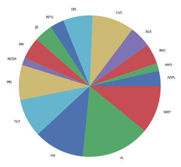
- Plotting the HRPOpt portfolio performance
hrp.portfolio_performance(verbose=True);
Expected annual return: 18.7%
Annual volatility: 19.1%
Sharpe Ratio: 0.87- Plotting the HRPOpt portfolio dendrogram
from pypfopt import plotting

plotting.plot_dendrogram(hrp); 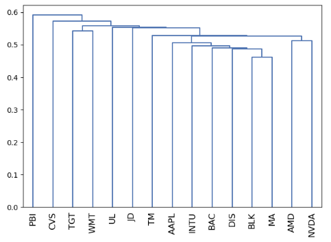
Discussion
- In this article, different aspects of the investment portfolio optimization (IPO) process were studied in great detail.
- We addressed the following two problems: (1) For a given portfolio return, we estimated portfolio weights that minimize the risk level of the portfolio; (2) For a given portfolio risk level, we determined portfolio weights that maximize the portfolio’s return.
- We tested both the traditional mean-variance (MV) optimization (Markowitz, 1952) and Black-Litterman (BL) IPO.
- The main focus was on the PyPortfolioOpt library that implements portfolio optimization methods, including classical efficient frontier techniques and BL allocation, as well as more recent developments in the field like shrinkage and Hierarchical Risk Parity.
Final Word
- In this study we implemented several IPO models in a multi-asset portfolio context.
- We have shown how multi-objective IPO be used efficiently in the decision support for investment portfolio planning under market uncertainty and friction.
- The resulting portfolios are less risky, are more diversified across asset classes, and have less extreme asset allocations.
- By analyzing stock historical data across multiple assets, objectives and time horizons, it is possible to quantitatively evaluate financial investments such as stocks and make correct investment decisions.
- Python largely facilitates the calculation of expected returns/variance, and can quickly find the optimal product, which is of great value for the asset portfolio management.
Explore More
- Stock Portfolio Risk/Return Optimization
- Risk/Return QC via Portfolio Optimization — Current Positions of The Dividend Breeder
- Portfolio Optimization Risk/Return QC — Positions of Humble Div vs Dividend Glenn
- Risk/Return POA — Dr. Dividend’s Positions
- Bear vs. Bull Portfolio Risk/Return Optimization QC Analysis
- Portfolio Optimization of 20 Dividend Growth Stocks
- Applying a Risk-Aware Portfolio Rebalancing Strategy to ETF, Energy, Pharma, and Aerospace/Defense Stocks in 2023
- Joint Analysis of Bitcoin, Gold and Crude Oil Prices
- Risk-Aware Strategies for DCA Investors
- Oracle Monte Carlo Stock Simulations
- A Market-Neutral Strategy
- Dividend-NG-BTC Diversify Big Tech
- IQR-Based Log Price Volatility Ranking of Top 19 Blue Chips
- Towards Max(ROI/Risk) Trading
- Top 6 Reliability/Risk Engineering Learnings
References
- Markowitz, Harry, 1952, Portfolio selection, Journal of Finance 7, 1, 77–91.
- Qullamaggie || Risk & Reward, Win Rate
- Portfolio optimization using Python
- An Introduction to Portfolio Optimization in Python
- Enhancing Investment Strategies Portfolio Optimization and Analysis
- Portfolio Optimization in Python 101 — SciPy edition
- Unlock the Power of AI-Driven Portfolio Optimization: Discover How DDPG and PPO Can Transform Your Investments
- Understanding Portfolio Optimization with Mean-Variance Analysis in Python
- Portfolio Optimization: The Black-Litterman Allocation Method
- Leveraging Python for Your Investment Portfolio Optimization
- MULTI-OBJECTIVE PORTFOLIO OPTIMISATION
- Portfolio Optimization using Python and Modern Portfolio Theory
- Portfolio Optimization: A Beginner’s Guide.
- Portfolio Optimization using Monte Carlo Simulation
- Optimize portfolio for max Sharpe ratio plot it out with efficient frontier curve
Contacts
Embed Socials
Infographics