Understanding Portfolio Optimization with Mean-Variance Analysis in Python

Portfolio optimization is a crucial aspect of investment strategy. It involves the selection of the best portfolio, out of the set of all portfolios being considered, according to some objective. The objective typically maximizes factors such as expected return and minimizes costs like financial risk.

Mean-variance analysis, introduced by Harry Markowitz in 1952, is a quantitative tool that allows investors to weigh these factors to select the most efficient portfolio. In this tutorial, we will delve into the intricacies of portfolio optimization using Python, focusing on mean-variance analysis to help you master the art of creating an optimized investment portfolio.

Prerequisites

Before we dive into the code, make sure you have the following Python libraries installed:

pip install yfinance numpy pandas matplotlib plotly mplfinance

These libraries will allow us to download financial data, perform numerical computations and create stunning visualizations.

Setting Up the Environment

To get started, we need to import the necessary libraries and set up our environment. We’ll use libraries like yfinance for data retrieval, numpy and pandas for numerical calculations, and matplotlib, plotly, and mplfinance for visualization.

import yfinance as yf
import numpy as np
import pandas as pd
import matplotlib.pyplot as plt
import plotly.graph_objects as go
import mplfinance as mpf

# Set the style for matplotlib
plt.style.use('seaborn-darkgrid')

Downloading Financial Data

We will use the yfinance library to download historical stock data for our analysis. For this tutorial, we will focus on a handful of financial assets.

# Define the ticker symbols for the assets we are interested in
assets = ['JPM', 'GS', 'MS', 'BLK', 'C']

# Download historical data for these assets until the end of November 2023
end_date = '2023-11-30'
data = yf.download(assets, end=end_date)['Adj Close']

# Display the first few rows of the data
print(data.head())

Exploratory Data Analysis

Before optimizing our portfolio, it’s essential to gain a better understanding of our data through exploratory data analysis (EDA). Let’s visualize the historical adjusted closing prices of the selected financial assets.

# Plot the historical adjusted closing prices
data.plot(figsize=(10, 7))
plt.title('Historical Adjusted Closing Prices')
plt.xlabel('Date')
plt.ylabel('Adjusted Close Price (USD)')
plt.legend(title='Ticker')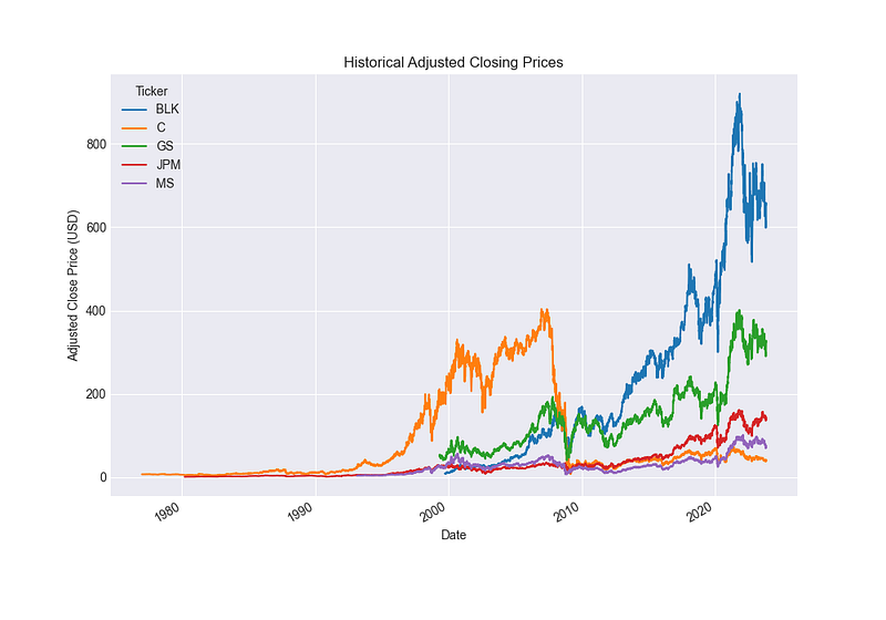

Figure 1: Historical adjusted closing prices of selected financial assets. Created by Author

Calculating Daily Returns

To perform mean-variance analysis, we need to calculate the daily returns of our assets.

# Calculate daily returns
daily_returns = data.pct_change().dropna()

# Plot the daily returns
daily_returns.plot(figsize=(10, 7))
plt.title('Daily Returns of Financial Assets')
plt.xlabel('Date')
plt.ylabel('Daily Returns')
plt.legend(title='Ticker')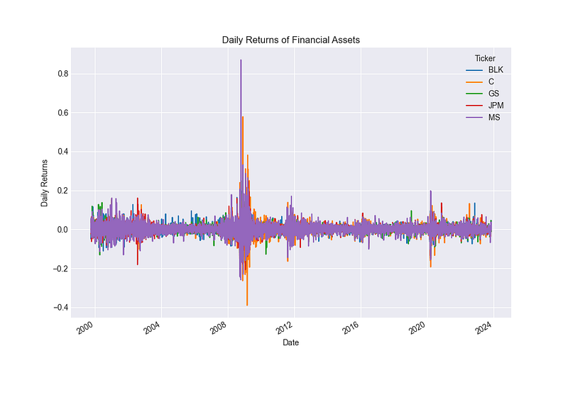

Figure 2: Daily returns of selected financial assets. Created by Author

Mean-Variance Analysis

Mean-variance analysis is based on the mean and variance of asset returns. Let’s calculate these for our portfolio.

# Calculate mean returns and covariance matrix
mean_returns = daily_returns.mean()
cov_matrix = daily_returns.cov()

# Display the mean returns and covariance matrix
print("Mean Returns:\n", mean_returns)
print("Covariance Matrix:\n", cov_matrix)

Building the Portfolio Optimization Model

Now, we will construct a Python class to encapsulate the logic of portfolio optimization. This class is designed to generate a diverse set of random portfolios and visualize the efficient frontier.

class PortfolioOptimizer:
    def __init__(self, returns, num_portfolios=10000, risk_free_rate=0.02):
        self.returns = returns
        self.num_portfolios = num_portfolios
        self.risk_free_rate = risk_free_rate
        self.assets = returns.columns
        self.num_assets = len(self.assets)
        self.portfolio_weights = []
        self.portfolio_expected_returns = []
        self.portfolio_volatilities = []
        self.portfolio_sharpe_ratios = []

    def generate_random_portfolios(self):
        np.random.seed(42)
        for _ in range(self.num_portfolios):
            weights = np.random.random(self.num_assets)
            weights /= np.sum(weights)
            self.portfolio_weights.append(weights)
            expected_return = np.sum(weights * self.returns.mean()) * 252
            self.portfolio_expected_returns.append(expected_return)
            volatility = np.sqrt(np.dot(weights.T, np.dot(self.returns.cov() * 252, weights)))
            self.portfolio_volatilities.append(volatility)
            sharpe_ratio = (expected_return - self.risk_free_rate) / volatility
            self.portfolio_sharpe_ratios.append(sharpe_ratio)

    def get_portfolio_performance(self, weights):
        weights = np.array(weights)
        expected_return = np.sum(weights * self.returns.mean()) * 252
        volatility = np.sqrt(np.dot(weights.T, np.dot(self.returns.cov() * 252, weights)))
        sharpe_ratio = (expected_return - self.risk_free_rate) / volatility
        return expected_return, volatility, sharpe_ratio

    def plot_efficient_frontier(self):
        portfolios = pd.DataFrame({
            'Return': self.portfolio_expected_returns,
            'Volatility': self.portfolio_volatilities,
            'Sharpe Ratio': self.portfolio_sharpe_ratios
        })

        # Plot efficient frontier
        plt.figure(figsize=(10, 7))
        plt.scatter(portfolios['Volatility'], portfolios['Return'], c=portfolios['Sharpe Ratio'], cmap='viridis')
        plt.colorbar(label='Sharpe Ratio')
        plt.xlabel('Volatility (Std. Deviation)')
        plt.ylabel('Expected Return')
        plt.title('Efficient Frontier')
        

        return portfolios

# Create an instance of PortfolioOptimizer
optimizer = PortfolioOptimizer(daily_returns)

# Generate random portfolios
optimizer.generate_random_portfolios()

# Plot the efficient frontier
portfolios = optimizer.plot_efficient_frontier()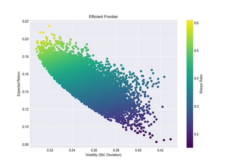

Figure 3: Efficient frontier of the randomly generated portfolios. Created by Author

Identifying the Optimal Portfolio

The optimal portfolio is the one that offers the highest Sharpe ratio. Let’s find it.

# Find the portfolio with the highest Sharpe ratio
optimal_idx = np.argmax(optimizer.portfolio_sharpe_ratios)
optimal_return = optimizer.portfolio_expected_returns[optimal_idx]
optimal_volatility = optimizer.portfolio_volatilities[optimal_idx]
optimal_weights = optimizer.portfolio_weights[optimal_idx]

print("Optimal Portfolio Weights:\n", optimal_weights)
print("Expected Annual Return: {:.2f}%".format(optimal_return * 100))
print("Annual Volatility / Std. Deviation: {:.2f}%".format(optimal_volatility * 100))
print("Sharpe Ratio:", max(optimizer.portfolio_sharpe_ratios))

Visualizing the Optimal Portfolio

Let’s visualize the optimal portfolio on the efficient frontier plot.

# Plot the efficient frontier with the optimal portfolio
plt.figure(figsize=(10, 7))
plt.scatter(portfolios['Volatility'], portfolios['Return'], c=portfolios['Sharpe Ratio'], cmap='viridis')
plt.colorbar(label='Sharpe Ratio')
plt.scatter(optimal_volatility, optimal_return, color='red', s=50) # Red dot
plt.xlabel('Volatility (Std. Deviation)')
plt.ylabel('Expected Return')
plt.title('Efficient Frontier with Optimal Portfolio')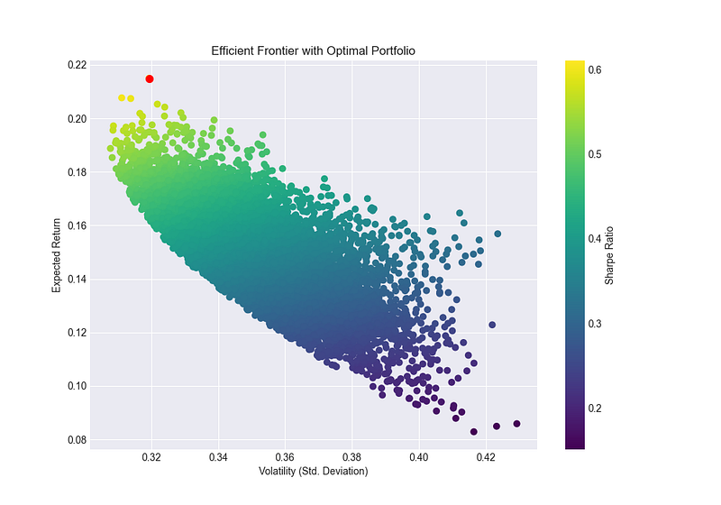

Figure 4: Efficient frontier with optimal portfolio. Created by Author

Conclusion

In this tutorial, we have explored the concept of portfolio optimization using mean-variance analysis in Python. We have covered the process of downloading financial data, performing exploratory data analysis, calculating daily returns, and constructing the efficient frontier. We have also implemented a class to encapsulate the portfolio optimization logic, which is a testament to the power of object-oriented programming in Python.

The optimal portfolio we identified offers the best risk-return trade-off according to the Sharpe ratio. This tutorial serves as a foundation for those interested in quantitative finance and provides a practical approach to portfolio optimization. With the skills you’ve learned here, you can extend this analysis to include more assets, different risk-free rates, or even alternative optimization techniques.

Remember, the journey to mastering portfolio optimization is ongoing, and there’s always more to learn and explore. Keep experimenting with different strategies and datasets to refine your investment approach.