
Portfolio Optimization: Using Python
Modern Portfolio Theory & Efficient Frontier
Background & Thoughts
What began with me wanting to put into practice some of the modern portfolio theory from CM2 led me to eventually write 250 lines of code to optimize some of my portfolio.
I currently have 3 of the mutual funds of the Mauritius Commercial Bank (MCB) in my personal portfolio which include the MCB Domestic Equites Fund (MCBDEF), the MCB Overseas Fund (MCBOF), and the MCB Yield Fund (MCBYF). My initial allocation dates back to 12 April 2022 which was purely on a discretionary basis (guilty of thinking I can just do so by interpreting factsheets). By 05 March 2023, my portfolio was down 3.743% (probably not a lot given recent market conditions but I must say it was kept fairly stable through dividend payments).
For full transparency, the initial allocation across the funds was 25% (MCBDEF), 40% (MCBOF), and 35% (MCBYF) which was me trying to “diversify” across both local and overseas holdings. Nevertheless, over the past few weeks, as I sit down exploring portfolio optimization techniques and building algorithms around historical data, I started writing down a few lines which could help me identify the optimal portfolio based on a certain set of constraints.
I have included some of the resources I have used as input (courtesy of ChatGPT). I have also commented out the full Python code which usually helps me find the logic behind a syntax and sometimes just a way to write down my thoughts. I now look forward to implementing this new risk-adjusted portfolio allocation and hopefully, it lives up to the claims of “long-term capital appreciation”.
Modern Portfolio Theory
Modern portfolio theory (MPT) is a mathematical framework for assembling a portfolio of assets such that risk-averse investors can construct portfolios to maximize expected return. This is based on a given level of market risk, emphasizing that higher risk is an inherent part of higher reward.
MPT uses weighted returns of equities to calculate a portfolio-wide return. Then it uses statistical measures such as variance (standard deviation) and correlation to determine ‘risk’ of a portfolio. It is important to note that for a portfolio comprised of ’n’ assets you can’t simply sum the standard deviation of each asset to calculate the total risk, but must also account for the correlation between assets.
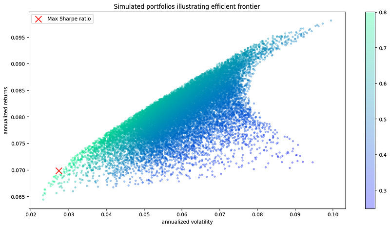
Using MPT, one can calculate what is called the ‘efficient frontier,’ which is the set of ‘optimal’ portfolios that offer the highest expected return for a defined level of risk. In this post, we will run thousands of portfolio simulations to highlight where the efficient frontier is, given a set of stocks.
The application of mean-variance portfolio theory is based on some important assumptions: all expected returns, variances and covariances of pairs of assets are known, investors make their decisions purely on the basis of expected return and variance, investors are non-satiated (prefers more to less), investors are risk-averse, and there are no taxes or transaction costs.
Code
import pandas as pd
import os.path
import glob
import matplotlib.pyplot as plt
import numpy as np
import datetime
import matplotlib.dates as mdates

# STEP I - GETTING THE DATA

# Define the folder path, Excel file names, and performance column names
folder_path = "C:\\Users\\Idjaz\\OneDrive\\Desktop\\Python\\MCB"
file_names = ['MCBGF.xlsx', 'MCBOF.xlsx', 'MCBYF.xlsx', 'MCBDEF.xlsx']
performance_names = ['MCBGF', 'MCBOF', 'MCBYF', 'MCBDEF']

# Read the first Excel file into a pandas DataFrame with the date column as the index (header = 5 since data only starts on the 5th row)
df = pd.read_excel(os.path.join(folder_path, file_names[0]), index_col='Ruling Date', header = 5)[['Performance Nav Dividend']]

# Rename the performance column based on the corresponding name in the list
df = df.rename(columns={'Performance Nav Dividend': performance_names[0]})

# Loop through the remaining Excel files (it takes the MCBGF dataframe as reference and loop through to take MCBOF and MCBYF as next)
for i in range(1, len(file_names)):
    # Read the Excel file into a pandas DataFrame with the date column as the index
    temp_df = pd.read_excel(os.path.join(folder_path, file_names[i]), index_col='Ruling Date', header = 5, usecols=['Ruling Date', 'Performance Nav Dividend'])

    # Rename the performance column based on the corresponding name in the list
    temp_df = temp_df.rename(columns={'Performance Nav Dividend': performance_names[i]})
    # Append the performance column to the main DataFrame
    df = pd.concat([df, temp_df], axis=1)

# Save the combined DataFrame to a new Excel file
#df = df.dropna(thresh=3) # for all dates that doesnt have 3 performance data points, it drops it to ensure consistency of data
df = df.drop(df.tail(9).index)
df.to_excel(os.path.join(folder_path,f"Data.xlsx"))

# STEP II - VISUALIZING THE DAILY PRICE DATA
df.index = pd.to_datetime(df.index)

fig = plt.figure(figsize=(14,7))
ax = fig.add_subplot(111)
# figsize: This is a tuple of two values that specifies the width and height of the figure in inches.
# In this case, (14, 7) means that the width of the figure will be 14 inches and the height will be 7 inches.

for i in df.columns.values:
    plt.plot(df.index, df[i],lw=2, alpha=0.8,label=i)
    # plt.plot(df.index, df[i], lw=2, alpha=0.8,label=i)
    # df.index: This is the x-axis data for the line plot. It is a pandas series representing the index of the DataFrame df. Here it is the Ruling Date.
    # lw=2: This argument sets the line width to 2. lw stands for "line width"
    # alpha=0.8: This argument sets the transparency of the line to 0.8. alpha stands for "alpha channel" which controls transparency
    # label=i: This argument sets the label of the line to i. i is the name of the column in df that is being plotted. This label will be used to create a legend for the line plot.

# since the axis is daily data for 10 years which makes it difficult to read the tickers, we are going to customize to show only every 2 years price data
ax.xaxis.set_major_locator(mdates.YearLocator(base=2))
ax.xaxis.set_major_formatter(mdates.DateFormatter('%Y'))

plt.title("Daily Price Data")
plt.legend(loc='upper left', fontsize=12) # determine position and fontsize of legend which here is upper left
plt.ylabel('Index NAV (MUR)') # y-axis label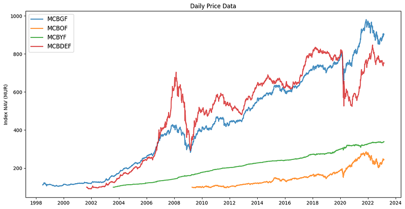
# STEP III - VISUALIZING THE DAILY % RETURN DATA

#Plotting this using daily % change in return can help illustrate the stocks' volatility.

returns = df.pct_change() #calculate the daily % return for each fund

fig = plt.figure(figsize=(14,7))
ax = fig.add_subplot(111)

for i in returns.columns.values:
    plt.plot(returns.index, returns[i], lw=2, alpha=0.8,label=i)

ax.xaxis.set_major_locator(mdates.YearLocator(base=2))
ax.xaxis.set_major_formatter(mdates.DateFormatter('%Y'))

plt.title("Daily % Return Data")
plt.legend(loc='upper left', fontsize=12)
plt.ylabel('daily returns (%)')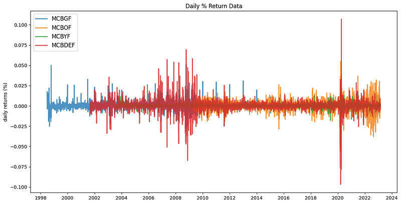
# STEP IV - DEFINING FORMULAS FOR SIMULATIONS

returns = df.pct_change() # computes the % daily returns based off the daily index price
mean_returns = returns.mean() # The mean() method in pandas DataFrame computes the mean of a set of variables.
cov_matrix = returns.cov() # The cov() method in pandas DataFrame computes the covariance matrix of a set of variables.
num_portfolios = 20000 # Number of portfolios to simulate
risk_free_rate = 0.0479

# Risk free rate (used for Sharpe ratio below)
# anchored on treasury bond rates - The value for the risk-free rate is based off the weighted average yield of Mauritius 10YR Bond Auction as of 11 Oct 2022 (4.79%)

# STEP V - DEFINING FUNCTIONS TO SIMULATE RANDOM PORTFOLIOS

# Define function to calculate returns, volatility
# The NYSE and NASDAQ average about 252 trading days a year (excludes holidays, weekends)

def portfolio_annualized_performance(weights, mean_returns, cov_matrix):

    # Return of portfolio
    returns = np.sum(mean_returns*weights) *252
    # mean_returns is a numpy array containing the mean expected returns for each asset in the portfolio,
    # while weights is a numpy array containing the portfolio weights for each asset.
    # The product of mean_returns and weights computes the expected return for each asset in the portfolio,
    # and then np.sum computes the sum of these expected returns to give the overall expected portfolio return.
    # Multiplying by 252 at the end converts the expected daily return to an expected annualized return, assuming 252 trading days in a year.

    # Standard deviation of portfolio
    std = np.sqrt(np.dot(weights.T, np.dot(cov_matrix, weights))) * np.sqrt(252)
    # In the context of portfolio optimization, covariance refers to the way in which the returns of different assets in the portfolio tend to move together.
    # A positive covariance indicates that the returns of the assets tend to move in the same direction, while a negative covariance indicates that the returns tend to move in opposite directions.
    # The covariance of two assets is influenced not only by their own individual volatility (i.e., standard deviation), but also by the degree to which they are related
    # to each other. If two assets have a high positive covariance, their combined volatility in a portfolio will be higher than if they had a low or negative covariance.
    # The inner product np.dot(cov_matrix, weights) computes the weighted covariance matrix of the portfolio returns.
    # In other words, it takes into account not only the covariance between the returns of the assets, but also the degree to which each asset contributes to the overall portfolio return.
    # The outer product np.dot(weights.T, np.dot(cov_matrix, weights)) computes the variance of the portfolio returns.
    # The square root of the portfolio variance gives the expected volatility of the portfolio,
    # which is then annualized by multiplying by the square root of the number of trading days in a year (assuming 252 trading days in a year).

    return std, returns

# STEP VI - GENERATING RANDOM PORTFOLIOS

def generate_random_portfolios(num_portfolios, mean_returns, cov_matrix, risk_free_rate):

    results = np.zeros((3,num_portfolios))
    # Initialize array of shape 3 x N to store our results
    # where N is the number of portfolios we're going to simulate
    # 3 rows: portfolio_std_dev, portfolio_return, and sharpe ratio
    # The array "results" has three rows and "num_portfolios" columns, all initialized to zero.
    # We will then use this array to store results or calculations for each portfolio in our analysis.

    weight_array = [] # Empty array to store the weights of each fund

    for i in range(num_portfolios):
        weights = np.random.random(4) # initializes a NumPy array called "weights" with four random weights (1 for each fund). Each time the code is ran, the numbers will be different because they are randomly generated.
        weights /= np.sum(weights) # Convert the randomized weights to percentages (summing to 100)
        weight_array.append(weights) # Add the generated random weights to the empty portfolio weight array/matrix above

        portfolio_std_dev, portfolio_return = portfolio_annualized_performance(weights, mean_returns, cov_matrix)
        # based off the random weights generated, it calls the portfolio annualized performance function and passes the weights to calculate the returns and std
        # it then returns the mean_returns (returns.mean()) and cov_matrix (returns.cov())

        results[0,i] = portfolio_std_dev
        results[1,i] = portfolio_return
        results[2,i] = (portfolio_return - risk_free_rate) / portfolio_std_dev # Sharpe ratio formula
        # In the above, the portfolio matrix is a 3 x N NumPy array where each column represents a different portfolio.
        # We then use the np.std function to calculate the standard deviation of each portfolio, resulting in a 1-dimensional NumPy array portfolio_std_devs with length N.
        # We then loop through each portfolio and store its standard deviation in the first row of the results array using the code results[0, i] = portfolio_std_devs[i].
        # Once this loop is finished, the results array will contain the standard deviation of each of the N portfolios.

    return results, weight_array

# STEP VII - RUNNING THE SIMULATIONS AND VISUALIZING THE DATA - OPTIMAL ALLOCATION

def display_simulated_portfolios(mean_returns, cov_matrix, num_portfolios, risk_free_rate):

    # pull results, weights from random portfolios
    results, weights = generate_random_portfolios(num_portfolios,mean_returns, cov_matrix, risk_free_rate)

    max_sharpe_idx = np.argmax(results[2])
    # pulls the max portfolio sharpe ratio (3rd element in results array from the generate_random_portfolios function)

    stdev_portfolio, returns_portfolio = results[0,max_sharpe_idx], results[1,max_sharpe_idx]
    # pulls the associated standard deviation, annualized return with respect to the the max Sharpe ratio

    max_sharpe_allocation = pd.DataFrame(weights[max_sharpe_idx],index=df.columns,columns=['allocation'])
    max_sharpe_allocation.allocation = [round(i*100,2)for i in max_sharpe_allocation.allocation]
    max_sharpe_allocation = max_sharpe_allocation.T
    # pulls the allocation associated with max Sharpe ratio and put it in a panda dataframe
    # rounds each element of the allocation attribute of the max_sharpe_allocation object to two decimal places and multiplies it by 100.
    # The DataFrame had 1 row and as many columns as there were assets in the portfolio. The row represented the allocation percentages of each asset in the portfolio.
    # By transposing the DataFrame with the .T method, the rows and columns are swapped.
    # This means that max_sharpe_allocation now has one column and as many rows as there are assets in the portfolio.
    # Each row represents the allocation percentage of a single asset in the portfolio.

    print("-"*100) # prints 100 times "-"
    print("Portfolio at maximum Sharpe Ratio\n") # leave a line after the print "\n"
    print("--Returns, volatility--\n")
    print("Annualized Return:", round(returns_portfolio,2)) # returns the return of the portfolio rounded to 2dp
    print("Annualized Volatility:", round(stdev_portfolio,2)) # returns the stdev of the portfolio rounded to 2dp

    print("\n")
    print("--Allocation at max Sharpe ratio--\n")
    print(max_sharpe_allocation)
    print("-"*100)

    plt.figure(figsize=(14, 7))
    # figsize: This is a tuple of two values that specifies the width and height of the figure in inches.
    # In this case, (14, 7) means that the width of the figure will be 14 inches and the height will be 7 inches.

    plt.scatter(results[0,:],results[1,:],c=results[2,:], cmap='winter', marker='o', s=10, alpha=0.3)
    # The plt.scatter function is used to create a scatter plot of three arrays of data.
    # The first array (results[0,:]) specifies the values for the x-axis, the second array (results[1,:]) specifies the values for the y-axis,
    # and the third array (results[2,:]) specifies the values to use for coloring the markers.
    # The size of each marker/circle is set to 10 (s=10), and the transparency of each marker is set to 0.3 (alpha=0.3).
    # The c argument of the plt.scatter function specifies the array to use for coloring the markers. In this case, the results[2,:] array is being used.
    # The cmap argument specifies the colormap to use for mapping the values in results[2,:] to colors (sharp ratio values)
    # In this case, the 'winter' colormap is being used, which maps lower values to blues and higher values to greens, yellows, and reds.
    # colourmaps directory can be found here: https://matplotlib.org/stable/tutorials/colors/colormaps.html
    # marker directory can be found here: https://matplotlib.org/stable/api/markers_api.html

    plt.colorbar()
    # In the context of the code you provided, plt.colorbar() is used to add a colorbar to the scatter plot created by plt.scatter().
    # The colorbar will show the mapping between the values in the results[2,:] array and the colors used to plot the markers.

    plt.scatter(stdev_portfolio, returns_portfolio, marker='x',color='r',s=150, label='Max Sharpe ratio')
    # The color argument specifies the color of the marker. In this case, 'r' is used to specify the color red.
    # The marker argument of the plt.scatter function specifies the marker to use for each data point in the scatter plot. In this case, red crosses ('x') are being used.
    # The plt.scatter function is used to create a scatter plot of two arrays of data.
    # The first array (stdev_portfolio) specifies the values for the x-axis, while the second array (returns_portfolio) specifies the values for the y-axis.

    plt.title('Simulated portfolios illustrating efficient frontier') # graph title
    plt.xlabel('annualized volatility') # x-axis label
    plt.ylabel('annualized returns') # y-axis label
    plt.legend(labelspacing=1.2) # The labelspacing argument of the plt.legend function specifies the spacing between the labels in the legend

display_simulated_portfolios(mean_returns, cov_matrix, num_portfolios, risk_free_rate)
New Risk-Adjusted Portfolio Allocation
----------------------------------------------------------------------------------------------------
Portfolio at maximum Sharpe Ratio

--Returns, volatility--

Annualized Return: 0.07
Annualized Volatility: 0.03

--Allocation at max Sharpe ratio--

            MCBGF  MCBOF  MCBYF  MCBDEF
allocation  19.01   0.19  75.88    4.92
----------------------------------------------------------------------------------------------------
Resources: