
Portfolio Optimization: The Black-Litterman Allocation Method
This article is the fourth chapter of a whole series on the use of Data Science for Stock Markets. I highly suggest you read the first chapter, “Introduction to Quant Investing with Python”, the second chapter, “The Science of Smart Investing: Portfolio Evaluation with Python”, and the third chapter “Portfolio Optimization: The Markowitz Mean-Variance Model”
I also recommend you read the notebook on Kaggle, 🤑 Data Science for Financial Markets 📈💰 for a better experience with the code, images, and plots.
Introduction
Developed by Fischer Black and Robert Litterman in 1992, the Black-Litterman Model works by taking a Bayesian approach to asset allocation. This model optimizes allocation weights by combining a prior estimate of returns, which can be derived from multiple sources, and incorporating the investor’s unique expectations for future returns.
At its core, the Black-Litterman model computes a weighted average of the prior estimates of returns and particular views held by the investor for each asset. The weighting is dictated by the confidence levels given by the investor for each of his views, which allows for a more personalized investment strategy.
Prior
A commonly used approach for determining a prior estimate of returns involves relying on the market’s expectations, which are reflected in the asset’s market capitalization.
To do this, we first need to estimate the level of risk aversion among market participants, represented by a parameter known as delta, which we compute by using the closing prices of the SP500. The higher the value for delta, the greater the market’s risk aversion.
Armed with this information, we can determine the initial expected returns for each stock. This calculation is based on three key factors: the stock’s market capitalization, the delta value representing market risk aversion, and the covariance matrix S. It’s important to remember that we derived this covariance matrix in our previous article where we optimized our portfolio using the Markowitz Mean-Variance Model. These prior expected returns give us a starting point for the expected returns before we incorporate any of our views as investors.
Views
In the Black-Litterman model, we can express our views as either absolute or relative. Absolute views involve statements like “APPL will return 10%”, while relative views are represented by statements such as “AMZN will outperform AMD by 10%”.
These views must be specified in the vector Q and mapped into each asset via the picking matrix P.
For instance, let’s consider a portfolio with the ten following assets:
1. TSLA
2. AAPL
3. NVDA
4. MSFT
5. META
6. AMZN
7. AMD
8. HD
9. GOOGL
10. BRKa
Let’s consider two absolute views and two relative views, such as:
1. TSLA will raise by 20%
2. APPL will drop by 15%
3. HD will outperform META by 10%
4. GOOGL and BRKa will outperform MSTF and AMZN by 5%
The views vector would be formed by taking the numbers above and specifying them as below:
Q = np.array([0.20, -0.15, 0.10, 0.05]).reshape(-1,1)
The picking matrix would then be used to link the views of the 8 mentioned assets above to our portfolio of 10 assets, allowing us to propagate our expectations into the model:
P = np.array([ [1,0,0,0,0,0,0,0,0,0],
[0,1,0,0,0,0,0,0,0,0],
[0,0,0,0,-1,0,0,1,0,0],
[0,0,0,-0.5,0,-0.5,0,0,0.5,0.5] ])
Absolute views have a single 1 in the column corresponding to the asset’s order in the asset universe, while relative views have a positive number in the outperforming asset column, and a negative number in the underperforming asset column. Each row for relative views in P must sum up to 0, and the order of views in Q must correspond to the order of rows in P.
Confidence Levels
The confidence matrix is used to help us define the allocations in each stock. It can be implemented using the Idzorek’s method, allowing investors to specify their confidence level in each of their views as percentage values. The values in the confidence matrix range from 0 to 1, where 0 indicates a low level of confidence in the view, and 1 indicates a high level of confidence.
By using the confidence matrix, investors can better understand the potential impact of their views on their allocations. For example, if an investor has a high level of confidence in their view on a particular asset’s performance, they may choose to allocate a larger portion of their portfolio to that asset. On the other hand, if an investor has a low level of confidence in their view, they may decide to allocate a smaller portion of their portfolio or avoid the asset altogether.
For more information on the Black-Litterman Allocation Model, I highly suggest you read this session on the PyPortfolioOpt documentation.
Optimizing Portfolio
Let’s begin by mapping the assets. Once mapped, we can obtain each company’s market cap through Yahoo.
# Mapping assets
assets = ['AAPL', 'TSLA', 'DIS', 'AMD']
# Obtaining market cap for stocks
market_caps = data.get_quote_yahoo(assets)['marketCap']
market_caps # Visualizing market caps for stocksAAPL 2518055124992 TSLA 624150380544 DIS 176707338240 AMD 155483013120 Name: marketCap, dtype: int64
We are going to obtain the market-implied risk aversion, our delta, by computing the .market_implied_risk_aversion with PyPortfolioOpt. It’s crucial to make it clear we are using prices in this case, instead of returns.
market_prices = yf.download("^GSPC",start = '2010-07-01',
                            end = '2023-02-11')['Adj Close']
delta = black_litterman.market_implied_risk_aversion(market_prices)
delta # Visualizing delta
3.3668161617990653
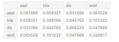
To visualize the prior estimates of returns, we are going to use the market caps and the delta we have obtained above, as well as the covariance matrix S we already have available from the previous notebook.
# Obtaining Prior estimates
prior = black_litterman.market_implied_prior_returns(market_caps,
                                                     delta, S)
prior # Visualizing prior estimates
AAPL 0.269523 TSLA 0.384137 DIS 0.141240 AMD 0.293677 dtype: float64
After obtaining the prior estimates of return for each one of the stocks, we can input our particular views for the stocks.
# Inputtig values for vector Q
Q = np.array([0.05,   # APPL will raise by 5%
              0.10,   # TSLA will raise by 10%
              0.15])  # AMD will outperform Disney by 15%
# Linking views to the P matrix
P = np.array([
[1,0,0,0], # APPL = 0.05
[0,1,0,0], # TSLA = 0.10
[0,0,-1,1] # AMD > DIS by 0.15
])Following on, we can create another vector called confidences, in which we inform the level of confidence we have in our views. These values range from 0 to 1, where values closer to 1 indicate higher confidence levels.
# Providing confidence levels
# Closer to 0.0 = Low confidence
# Closer to 1.0 = High confidence
confidences = [0.5,
               0.4,
               0.8]
After that, we can create the model.
# Creating model
bl = BlackLittermanModel(S, # Covariance Matrix
                         pi = prior, # Prior expected returns
                         Q = Q, # Vector of views
                         P = P, # Matrix mapping the views
                         omega = 'idzorek', # Confidence levels in %
                         view_confidences = confidences) # Confidences

rets = bl.bl_returns() # Calculating Expected returns
ef = EfficientFrontier(rets, S) # Optimizing asset allocation

ef.max_sharpe() # Optimizing weights for maximal Sharpe ratio
weights = ef.clean_weights() # Cleaning weights
weights # Printing weights
OrderedDict([('AAPL', 0.63718),
('TSLA', 0.18636),
('DIS', 0.01442),
('AMD', 0.16204)])By using the max_sharpe() function, we optimize the allocation weights for the maximum value for the Sharpe ratio. With these conditions, the Black-Litterman Model returned us a portfolio with the following weight allocation:
63.71% for Apple (AAPL).
18.63% for Tesla (TSLA).
1.44% for Disney (DIS).
1.62% for AMD (AMD).
Evaluating Optimized Portfolio
Now that we have the optimal allocation weights for the maximum Sharpe ratio, we can construct our Black-Litterman optimized portfolio.
# Building Black-Litterman portfolio
# Defining weights
black_litterman_weights = [0.62588,
                           0.19951,
                           0.016,
                           0.15861]

# Mapping each weight to each stock
black_litterman_portfolio = aapl*black_litterman_weights[0] +
                            tsla*black_litterman_weights[1] +
                            dis*black_litterman_weights[2] +
                            amd*black_litterman_weights[3]
By using the Quantstats library report, we can compare the Black-Litterman portfolio to the original portfolio we have built in this article.
# Comparing Black-Litterman portfolio to the original portfolio
qs.reports.full(black_litterman_portfolio, benchmark = portfolioo
Performance Metrics Strategy Benchmark ------------------------- ---------- ----------- Start Period 2010-07-01 2010-07-01 End Period 2023-02-10 2023-02-10 Risk-Free Rate 0.0% 0.0% Time in Market 100.0% 100.0% Cumulative Return 4,105.09% 3,429.90% CAGR﹪ 34.48% 32.62% Sharpe 1.15 1.08 Prob. Sharpe Ratio 100.0% 99.99% Smart Sharpe 1.09 1.03 Sortino 1.68 1.58 Smart Sortino 1.6 1.51 Sortino/√2 1.19 1.12 Smart Sortino/√2 1.13 1.06 Omega 1.22 1.22 Max Drawdown -45.36% -52.21% Longest DD Days 481 404 Volatility (ann.) 29.68% 30.59% R^2 0.89 0.89 Information Ratio 0.01 0.01 Calmar 0.76 0.62 Skew -0.18 -0.08 Kurtosis 3.71 3.9 Expected Daily % 0.12% 0.11% Expected Monthly % 2.49% 2.37% Expected Yearly % 30.61% 28.99% Kelly Criterion 9.35% 7.94% Risk of Ruin 0.0% 0.0% Daily Value-at-Risk -2.94% -3.04% Expected Shortfall (cVaR) -2.94% -3.04% Max Consecutive Wins 13 13 Max Consecutive Losses 8 8 Gain/Pain Ratio 0.22 0.21 Gain/Pain (1M) 1.44 1.35 Payoff Ratio 0.97 0.97 Profit Factor 1.22 1.21 Common Sense Ratio 1.28 1.26 CPC Index 0.65 0.64 Tail Ratio 1.05 1.04 Outlier Win Ratio 3.72 3.6 Outlier Loss Ratio 3.5 3.44 MTD 7.19% 6.71% 3M 16.89% 22.42% 6M -15.01% -14.88% YTD 26.4% 31.62% 1Y -20.82% -26.29% 3Y (ann.) 40.43% 35.01% 5Y (ann.) 42.34% 39.74% 10Y (ann.) 38.88% 38.55% All-time (ann.) 34.48% 32.62% Best Day 11.5% 13.76% Worst Day -13.75% -12.65% Best Month 30.35% 30.34% Worst Month -18.08% -19.49% Best Year 165.75% 172.25% Worst Year -39.67% -47.22% Avg. Drawdown -4.22% -4.46% Avg. Drawdown Days 25 27 Recovery Factor 90.49 65.7 Ulcer Index 0.12 0.13 Serenity Index 26.63 19.5 Avg. Up Month 8.96% 8.86% Avg. Down Month -6.18% -6.51% Win Days % 55.38% 54.72% Win Month % 61.84% 61.18% Win Quarter % 74.51% 66.67% Win Year % 92.86% 92.86% Beta 0.91 - Alpha 0.04 - Correlation 94.09% - Treynor Ratio 4497.23% -
By using the Black-Litterman Allocation Model, we were able to improve our portfolio’s performance metrics compared to the original portfolio, where each asset was given a uniform weight of 25%. The Black-Litterman optimized portfolio outperformed the original portfolio in several key metrics. First, it generated higher Cumulative Return and CAGR, indicating a stronger performance. Additionally, the Sharpe and Sortino ratios were higher, demonstrating superior risk-return relationship.
The optimized portfolio also has a lower maximum drawdown and annual volatility compared to the original portfolio, implying less downside risk and more stability to the optimized portfolio. In terms of expected returns, the Black-Litterman portfolio shows higher daily, monthly, and yearly returns, and lower Daily Value-at-Risk, indicating a lower risk of significant losses in a given day.
The optimized portfolio also has lower averaged drawdown and higher recovery factor, meaning it bounces back faster from losses, and the beta of the optimized portfolio was much lower than that of the original portfolio, indicating lower market risk. Overall, the Black-Litterman optimized portfolio achieved higher returns at lower risks compared to the first portfolio we have built.
Conclusion
Both the Markowitz Mean-Variance Model and the Black-Litterman Allocation Model effectively enhanced performance and reduced the risks associated with the original portfolio by optimizing the allocation weights of Apple, Tesla, Disney, and AMD stocks.
The Markowitz optimization resulted in a portfolio that primarily invested in Apple and a smaller portion in Tesla, with no allocation in Disney and AMD. On the other hand, the Black-Litterman optimization allocated funds into all four stocks, but still favored Apple with the majority of the allocation.
The preference for Apple in both optimizations is not coincidental. Our initial analysis, performed in this article, did reveal that Apple had the highest Sharpe ratio, lowest beta, and demonstrated superior performance with lower risk compared to the other stocks.
It’s also interesting to compare the two optimized portfolios. The Markowitz optimized portfolio outperformed the Black-Litterman portfolio in terms of Cumulative Returns, CAGR, Sharpe ratio, Profit Factor, Recovery Factor, and overall performance. On the other hand, the Black-Litterman portfolio demonstrated some advantages, such as lower drawdown, lower annual volatility, and better performance on its worst day and worst month.
In conclusion, portfolio optimization is a very important step to improve the risk-return relationship of a portfolio by adjusting its asset allocation. By using various mathematical models and optimization techniques, it’s possible to efficiently improve performance and reduce the exposure to risk.
While there are different approaches to portfolio optimization, including the Markowitz Mean-Variance model and the Black-Litterman allocation model, there is no one-size-fits-all solution. The choice of the model to use depends on each investor’s personal risk tolerance, investment goals, horizon of investment, as well as market conditions.
To gain a deeper understanding of portfolio optimization, you can explore many research papers, journals, and books on the subject. Some sources of research to consider include books such as Modern Portfolio Theory and Investment Analysis by Edwin J. Elton and Martin Jay Gruber, Portfolio Selection by Harry Markowitz, and Active Portfolio Management: A Quantitative Approach for Producing Superior Returns and Controlling Risk by Richard C. Grinold and Ronald N. Kahn, which can provide valuable insights into the theory and practice of portfolio optimization.
Thank you for reading.
Luis Fernando Torres
Let’s connect!🔗 LinkedIn • Kaggle • HuggingFace
Like my content? Feel free to Buy Me a Coffee ☕ !
A Message from InsiderFinance

Thanks for being a part of our community! Before you go:
- 👏 Clap for the story and follow the author 👉
- 📰 View more content in the InsiderFinance Wire
- 📚 Take our FREE Masterclass
- 📈 Discover Powerful Trading Tools


