Introduction to Quant Investing with Python

Introduction

Data Science is a rapidly growing field in the current global scenario, combining the power of Statistics with computational techniques to obtain valuable insights from data. Data Scientists are professionals responsible for integrating knowledge from various fields such as Mathematics, Statistics, Computer Science, and domain-specific knowledge to identify patterns and extract information from large volumes of data, whether structured or unstructured. With this information, it becomes possible to find solutions to help in decision-making in business, investments, scientific research, and public policy.

When it comes to financial markets, Data Science can be applied in various ways, such as:

• Predictive Models: Data Science professionals can use historical data to create predictive models that can identify trends and make predictions about future market conditions;
• Algorithmic Trading: The use of algorithms that execute buy and sell orders autonomously, based on mathematical models through the analysis of price, volume, and volatility, among many others;
• Portfolio Optimization: Algorithms and other mathematical models can be used to optimize portfolios, aiming for maximization of returns and risk minimization;
• Fraud Detection: Machine learning algorithms can identify fraudulent activities in financial transactions;
• Risk Management: Data Science can be used to quantify and facilitate the management of various financial risks, including market risk, credit risk, and operational risk;
• Customer Analysis: Financial institutions can use Data Science to analyze customer data and obtain information about their behavior and preferences, which can help to improve customer relations and retention.

In this introductory article, I intend to demonstrate how Data Science and Python can be powerful tools to obtain market insights and improve the performance of your investments through portfolio optimization, the development of efficient investment strategies, and stock analysis.

Quantstats

Quantstats is a Python library used for quantitative financial analysis and portfolio optimization. This library provides various tools to obtain financial data from different sources, conduct technical and fundamental analyses, and create and test investment strategies. It is also possible to use visualization tools to analyze stocks and portfolios. Quantstats is a simple and easy tool for quantitative finance-oriented analysis, and that’s why it will be the library of choice for this study. To install Quantstats on your computer, use the following command in any Python environment:

# Installing Quantstat

!pip install quantstats

After that, you may import some essential libraries.

# Importing libraries
import pandas as pd
import numpy as np
import quantstats as qs
import matplotlib.pyplot as plt
import seaborn as sns
from sklearn.linear_model import LinearRegression
import plotly.express as px
import yfinance as yf

After installing and importing quantstats, we must load the data of the stocks we want to analyze. In this case, I decided to analyze Apple, Tesla, The Walt Disney Company, and AMD stocks, in a period going from July 1st, 2010 to February 10th, 2023. We can use quantstats method download_returns to obtain the daily returns data.

# Getting daily returns for 4 different US stocks in the same time window
aapl = qs.utils.download_returns('AAPL')
aapl = aapl.loc['2010-07-01':'2023-02-10']
 
tsla = qs.utils.download_returns('TSLA')
tsla = tsla.loc['2010-07-01':'2023-02-10']
 
dis = qs.utils.download_returns('DIS')
dis = dis.loc['2010-07-01':'2023-02-10']
 
amd = qs.utils.download_returns('AMD')
amd = amd.loc['2010-07-01':'2023-02-10']

We now have aapl, tsla, dis, and amd variables, containing data from four different US stocks from different industries.

We may now start to take a look at a few metrics!

Cumulative Returns

Cumulative returns represent the total returns of an investment. When looking at stocks, it includes not only the appreciation of the stock’s price on the market but also dividends and any other form of income received.

Generally, cumulative returns are expressed as a percentage, and you can calculate it by obtaining the stock’s initial price and its final price at the end of the specified period. Then you subtract the initial price from the final price, add any dividends or other income received, and divide the result by the initial price. This gives us the cumulative return as a decimal, which can be multiplied by 100 to express it as a percentage.

Below, you can see a line chart displaying the cumulative returns for each one of the stocks we’ve downloaded since July 2010.

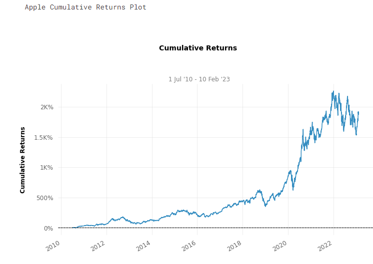
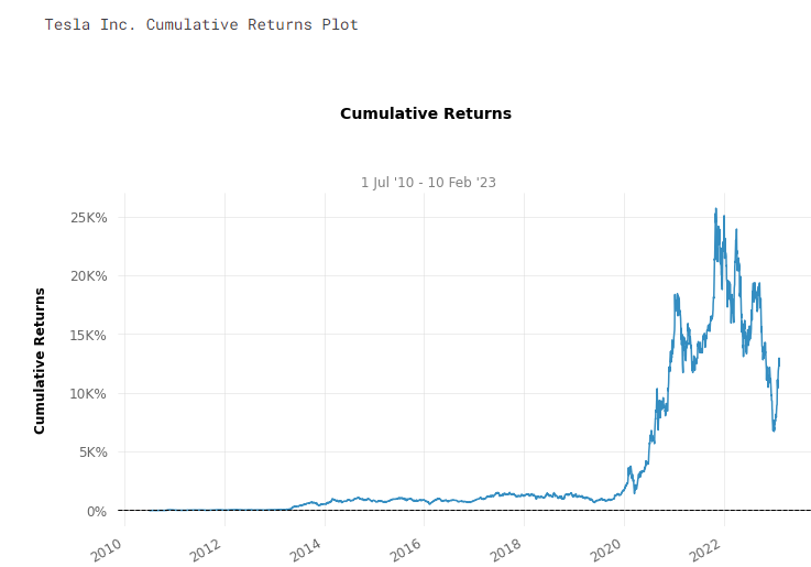
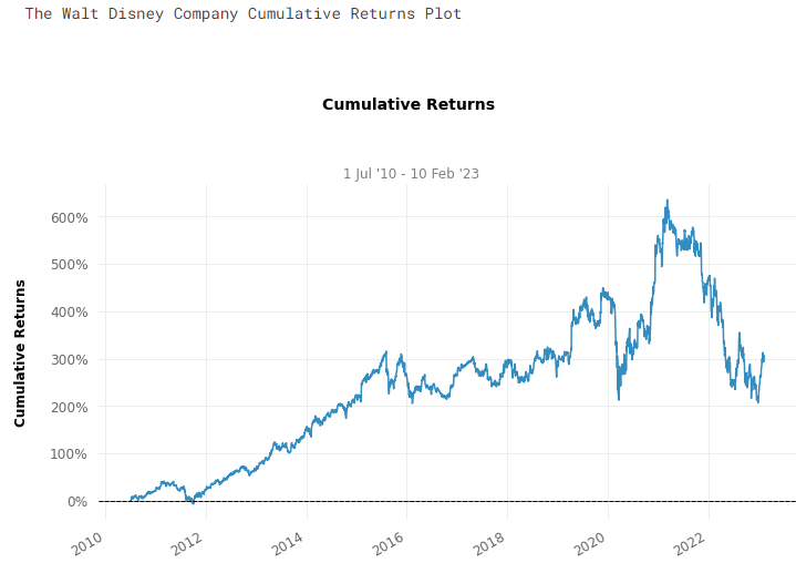
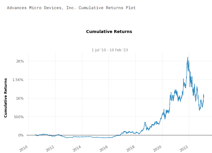
Observing the charts above, it’s possible to extract some interesting insights. For instance, you can see a considerable difference between Tesla’s and Disney’s returns. At the peak of its returns, Tesla surpassed an incredible mark of over 25,000%, which was a remarkable investment for those who had the foresight to buy the company’s shares by the beginning of the decade. On the other hand, Disney’s shares had some modest returns, peaking at around 650%.

Of course, when analyzing past data, we don’t make investment decisions looking only at the cumulative returns. It’s crucial to look at other indicators and evaluate the risks of an investment. Besides, 650% returns are still significant, and in the stock market, slow but steady growth can be just as valuable as explosive returns.

To build a robust portfolio, it’s important to consider a variety of strategies and characteristics of many different assets.

Daily Returns

Daily returns display the percentual change in stock prices over the day. It can be obtained by subtracting the current day closing from the previous close and then dividing it by the previous close. To express it as a percentage, you simply multiply the result by 100.

With quantstats, we can easily plot the daily returns over the period. For investors, looking at daily returns may be helpful to observe how prices behave in the market, allowing them to extract information on volatility and consistency of returns.

With the code below, we plot daily returns for each stock.

# Plotting Daily Returns for each stock
print('\nApple Daily Returns Plot:\n')
qs.plots.daily_returns(aapl)
print('\nTesla Inc. Daily Returns Plot:\n')
qs.plots.daily_returns(tsla)
print('\nThe Walt Disney Company Daily Returns Plot:\n')
qs.plots.daily_returns(dis)
print('\nAdvances Micro Devices, Inc. Daily Returns Plot:\n')
qs.plots.daily_returns(amd)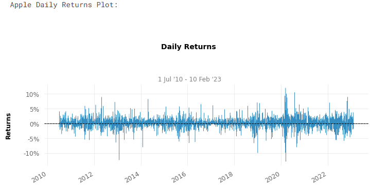

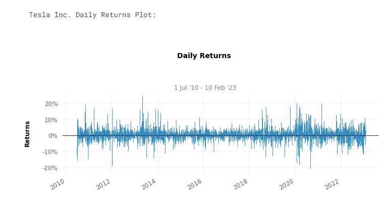
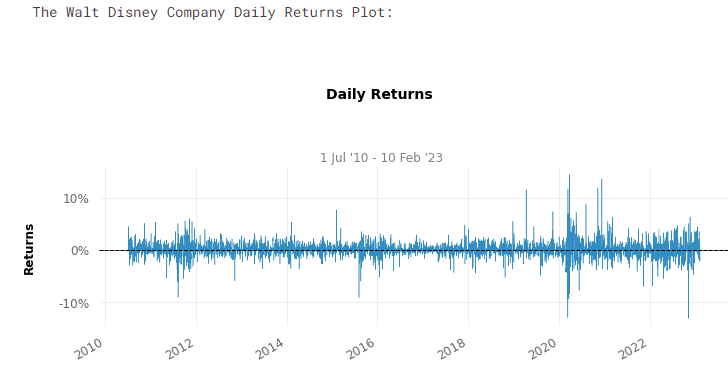
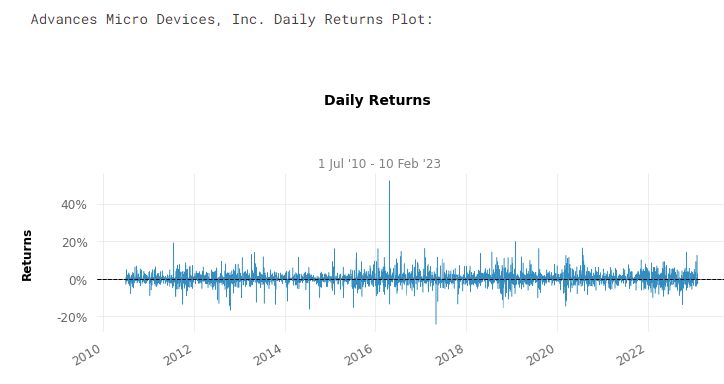
The plots above allow us to see an unusual variation in AMD stock prices, an increase of around 40% in its shares by 2016, which may have occurred for various factors, such as surprising earnings reports, increased demand for the company’s products, or favorable market conditions. This kind of behavior may indicate high volatility. Thus, marking it a riskier investment. On the other hand, Disney’s and Apple’s stocks seem more stable and predictable investment options.

Histograms

Histograms are a graphical representation of the distribution of values in a dataset, displaying how frequent they are.

Histograms of daily returns are valuable to help investors to identify patterns, such as the range of daily returns of an asset over a certain period, indicating its level of stability and volatility.

Once again, we may use quantstats to plot histograms of the analyzed assets.

# Plotting histograms
print('\nApple Daily Returns Histogram')
qs.plots.histogram(aapl, resample = 'D')
 
print('\nTesla Inc. Daily Returns Histogram')
qs.plots.histogram(tsla, resample = 'D')
 
print('\nThe Walt Disney Company Daily Returns Histogram')
qs.plots.histogram(dis, resample = 'D')
 
print('\nAdvances Micro Devices, Inc. Daily Returns Histogram')
qs.plots.histogram(amd, resample = 'D')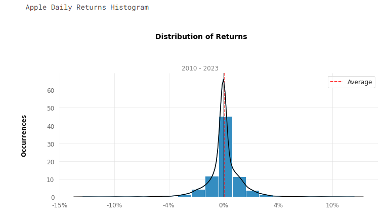

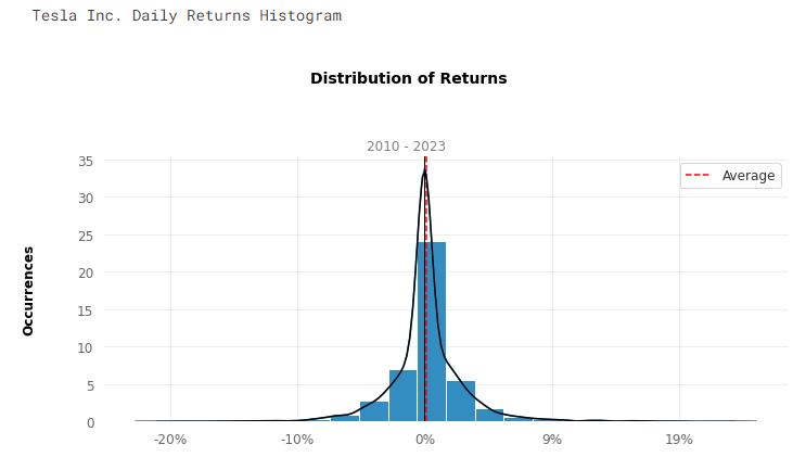
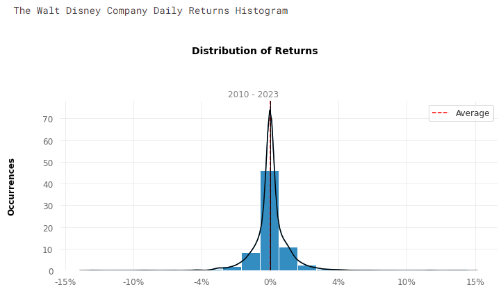
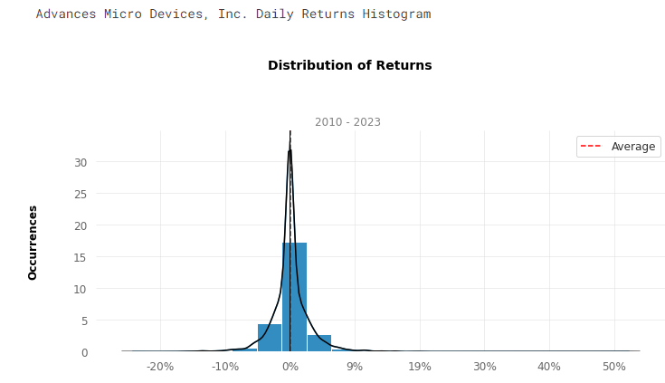
Through the analysis of the histograms, we can observe that most daily returns are close to zero in the center of the distribution. However, it’s easy to see some extreme values that are distant from the mean, which is the case of AMD, with daily returns of around 50%, indicating the presence of outliers in the positive range of the distribution. In contrast, in the negative field, it seems to have a limit of about -20%.

Disney’s stocks seem to display more balanced returns, with values ranging from -15% and 15%, while most of its returns are closer to the mean.

Using histograms, we can extract some valuable statistics such as kurtosis and skewness.

Kurtosis

A high kurtosis value for daily returns may indicate frequent fluctuations in price that deviate significantly from the average returns of that investment, which can lead to increased volatility and risk associated with the stock.

A kurtosis value above 3.0 is called a leptokurtic distribution, characterized by outliers and more values that are distant from the average, which reflects in the histogram as stretching of the horizontal axis. Stocks with a leptokurtic distribution are generally associated with a higher level of risk but also offer the potential for higher returns due to the substantial price movements that have occurred in the past.

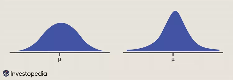
In the image below, it’s possible to see the difference between a negative kurtosis, on the left, and a positive kurtosis, on the right. The distribution on the left displays a lower probability of extreme values and lower concentration of values around the mean, while the distribution on the right shows a higher concentration of values near the mean, but also the existence, and thus a higher probability of occurrence, of extreme values.

Kurtosis

Kurtosis measures the concentration of observations in the tails versus the center of a distribution. In finance, a high level of excess kurtosis, or “tail risk,” represents the chance of a loss occurring as a result of a rare event. This type of risk is important for investors to consider when making investment decisions, as it may impact a particular stock’s potential returns and stability.

Once again, we use quantstats to measure the kurtosis of the analyzed stocks.

# Using quantstats to measure kurtosis
print("Apple's kurtosis: ", qs.stats.kurtosis(aapl).round(2))
print("Tesla's kurtosis: ", qs.stats.kurtosis(tsla).round(2))
print("Walt Disney's kurtosis: ", qs.stats.kurtosis(dis).round(3))
print("Advances Micro Devices' kurtosis: ", qs.stats.kurtosis(amd).round(3))

Apple's kurtosis:  5.26
Tesla's kurtosis:  5.04
Walt Disney's kurtosis:  11.033
Advances Micro Devices' kurtosis:  17.125

The kurtosis values above show that all four stocks, Apple, Tesla, Walt Disney, and Advanced Micro Devices, have high levels of kurtosis, which indicates a concentration of observations in the tails of their daily returns’ distributions, suggesting that all four stocks are subject to high levels of volatility and risk, with large price fluctuations that deviate significantly from their average returns.

However, AMD has the highest kurtosis, with a value of 17.125, indicating that AMD is subject to an extremely high level of tail risk, with a large concentration of extreme price movements. On the other hand, Disney has a kurtosis of 11.033, which is still higher than a typical value for a normal distribution, but not as extreme as AMD’s.

Skewness

Skewness is a metric that quantifies the asymmetry of returns. It reflects the shape of the distribution and determines if it is symmetrical, skewed to the left, or skewed to the right.

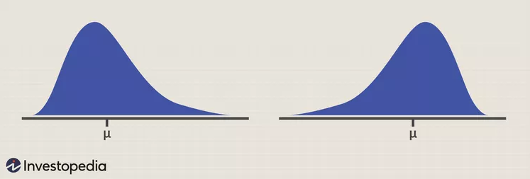
Below, it is possible to see two different asymmetrical distributions. On the left, it shows an example of a positively skewed distribution, with a long right tail, indicating a bigger probability of extremely positive daily returns when compared to a normal distribution. On the other hand, a negatively skewed distribution would most likely resemble the distribution on the right, with a long tail representing a bigger frequency of outliers on the negative side of returns.

Skewness

When skewness is equal to zero, it indicates a symmetrical distribution, where both tails are about the same size, and values are equally distributed on both sides of the mean.

With quantstats, and python, we calculate skewness as below:

# Measuring skewness with quantstats
print("Apple's skewness: ", qs.stats.skew(aapl).round(2))
print("Tesla's skewness: ", qs.stats.skew(tsla).round(2))
print("Walt Disney's skewness: ", qs.stats.skew(dis).round(3))
print("Advances Micro Devices' skewness: ", qs.stats.skew(amd).round(3))

Apple's skewness:  -0.07
Tesla's skewness:  0.33
Walt Disney's skewness:  0.199
Advances Micro Devices' skewness:  1.043

Generally, a value between -0.5 and 0.5 indicates a slight level of skewness, while values below -1 and above 1 are indications of strong asymmetry.

Apple, Tesla, and Disney are slightly skewed, and Disney’s slight skewness can be seen by looking at the range of the x-axis of its histogram, balanced between -15% and 15%.

AMD stocks are strongly positively skewed, which can also be easily identifiable by looking at the range between -20% and 50% in its histogram. AMD has a lot of outliers on the positive tail, which could’ve been a good thing for those who bought its shares but also exhibit higher volatility and risk to this investment.

Standard Deviation

Standard deviation is a widely used statistical metric that quantifies the variability of the dataset. When applied to a stock’s daily returns, it can indicate the risk level associated with investing in that particular stock. A stock exhibiting high daily return volatility, characterized by a high standard deviation, is considered riskier when compared to one with low daily return volatility, represented by a low standard deviation.

Standard deviation enables investors to assess the risk level and to compare the volatility of different stocks. For instance, if two assets have similar average returns, but one has a higher standard deviation, it is usually considered a riskier investment. Hence, standard deviation serves as a useful tool in helping investors make informed decisions regarding their investment choices and portfolio management.

Here’s how to obtain the standard deviation of a dataset with Python:

# Calculating Standard Deviations
print("Apple's Standard Deviation from 2010 to 2023: ", aapl.std().round(3))
print("\nTesla's Standard Deviation from 2010 to 2023: ", tsla.std().round(3))
print("\nDisney's Standard Deviation from 2010 to 2023: ", dis.std().round(3))
print("\nAMD's Standard Deviation from 2010 to 2023: ", amd.std().round(3))

Apple's Standard Deviation from 2010 to 2023:  0.018
 
Tesla's Standard Deviation from 2010 to 2023:  0.036
 
Disney's Standard Deviation from 2010 to 2023:  0.016
 
AMD's Standard Deviation from 2010 to 2023:  0.036

Based on the values above, we can say that Apple and Disney are less volatile than Tesla and AMD, suggesting that Apple and Disney are safer investment options, exhibiting smaller price fluctuations in the market.

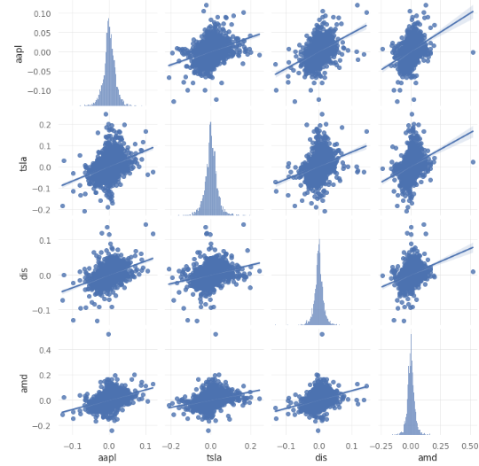
Pairplots and Correlation Matrix

Correlation analysis in the stock market allows us for interesting investment strategies. A widely known strategy in the market is called Long-Short, which is the act of buying shares of a company, while selling shares of another company, believing that both assets will have opposite directions in the market. That is, when one goes up, the other goes down. To develop Long-Short strategies, investors rely on correlation analysis between stocks.

Correlation analysis is not only useful for Long-Short strategies, but it’s also crucial to avoid systemic risk, which is described as the risk of the breakdown of an entire system rather than simply the failure of individual parts. To make it simple, if your portfolio has stocks that are highly correlated, or are all in the same industry if something happens to that specific industry, all of your stocks may lose market value and cause greater financial losses.

Pairplots and correlation matrices are useful tools to visualize correlation among assets. In the correlation matrix, values range between -1 and 1, where -1 represents a perfect negative correlation and 1 represents a perfect positive correlation. Keep in mind that, when assets are positively correlated, they tend to go up and down simultaneously in the market, while the opposite is true for those that are negatively correlated.

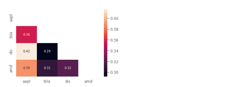
The stronger correlation among the assets above is between Disney and Apple. However, a correlation of 0.42 is not a strong one.

It’s important to note that there is not any negative correlation among the assets above, which indicates that none of them acts to limit losses. In the financial market, a hedge is an investment position intended to offset potential losses by investing in assets that may have a negative correlation with the others in a portfolio. Many investors buy gold to serve as protection for riskier investments, such as stocks, and when the market as a whole goes into a bear market, the gold tends to increase in value, limiting potential losses.

Beta and Alpha

Beta and Alpha are two key metrics used in finance to evaluate the performance of a stock relative to the overall market. Beta is a measure of a stock’s volatility compared to the market. A Beta of 1 means that the stock is as volatile as the market, a Beta greater than 1 indicates higher volatility than the market, and a Beta less than 1 suggests lower volatility.

Alpha, on the other hand, is a measure of a stock’s excess return relative to its expected performance based on its Beta. A positive Alpha indicates that a stock has outperformed its expected performance based on its Beta, while a negative Alpha suggests underperformance. By analyzing the Beta and Alpha values of stocks, investors can get a better understanding of the risk and potential returns of the stock compared to the market, and make informed investment decisions accordingly.

To determine Beta and Alpha, we require data from the SP500, which acts as the benchmark, to fit a linear regression model between the stocks and the index. This will enable us to extract the Beta and Alpha values of the stocks.

First, we load data on the SP500:

# Loading data from the SP500, the american benchmark
sp500 = qs.utils.download_returns('^GSPC')
sp500 = sp500.loc['2010-07-01':'2023-02-10']
sp500.index = sp500.index.tz_convert(None)

After that, we can use the Scikit-Learn Linear Regression model to extract Beta and Alpha.

# Fitting linear relation among Apple's returns and Benchmark
X = sp500_no_index.values.reshape(-1,1)
y = aapl_no_index.values.reshape(-1,1)
 
linreg = LinearRegression().fit(X, y)
 
beta = linreg.coef_[0]
alpha = linreg.intercept_
 
print('AAPL beta: ', beta.round(3))
print('\nAAPL alpha: ', alpha.round(3))

Doing that with the other stocks, this is what we have:

AAPL beta: [1.111]
AAPL alpha: [0.001]

TSLA beta: [1.377]
TSLA alpha: [0.001]
 
Walt Disney Company beta: [1.024]
Walt Disney Company alpha: [0.0001]
 
AMD beta: [1.603]
AMD alpha: [0.0006]

Beta values for all the stocks are greater than 1, meaning that they are more volatile than the benchmark and may offer higher returns, but also come with higher risk. On the other hand, the alpha values for all the stocks are small, close to zero, suggesting that there is little difference between the expected returns and the risk-adjusted returns.

Sharpe Ratio

The Sharpe Ratio is a metric that allows us to calculate the risk-return relation of an investment. You can calculate it as shown in the image below:

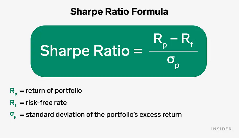
The risk-free rate of return is typically represented by a government bond.

A higher Sharpe ratio indicates that an investment provides higher returns for a given level of risk compared to other investments with a lower Sharpe ratio. In general, a Sharpe ratio above 1.0 is considered acceptable or good, 2.0 or higher is rated as very good, and 3.0 or higher is considered excellent. A Sharpe ratio of 1 means that the investment’s average return is equal to the risk-free rate of return.

With quantstats, this is how you obtain the Sharpe ratio of stocks:

# Calculating Sharpe ratio
print("Sharpe Ratio for AAPL: ", qs.stats.sharpe(aapl).round(2))
print("Sharpe Ratio for TSLA: ", qs.stats.sharpe(tsla).round(2))
print("Sharpe Ratio for DIS: ", qs.stats.sharpe(dis).round(2))
print("Sharpe Ratio for AMD: ", qs.stats.sharpe(amd).round(2))

Sharpe Ratio for AAPL:  0.97
Sharpe Ratio for TSLA:  0.95
Sharpe Ratio for DIS:  0.55
Sharpe Ratio for AMD:  0.62

Apple and Tesla have the highest Sharpe ratios among the four stocks analyzed, 0.97 and 0.95, respectively, indicating that these investments offer a better risk-return relationship. However, none of the stocks have a Sharp ratio above 1, which may indicate that these investments’ average returns are beneath the risk-free rate of return.

It’s important to note that the Sharpe ratio is an annual metric and since the beginning of 2022, the market, in general, has been bearish, with prices going down over the past year.

Initial Conclusions

Some conclusions can be drawn via the analysis of the metrics above:

• Apple and Tesla have the best Sharpe ratios, which indicates a better risk-return relationship;
• Tesla has the highest returns of them all, but it’s also more volatile than Apple and Disney;
• Apple has higher returns and low volatility compared to the other assets. It has the best Sharpe ratio, low beta, low standard deviation, and low asymmetry of returns;
• AMD is the riskier and more volatile investment option of the four. Its returns distribution is highly asymmetric, it has a high standard deviation value and high beta;
• Disney stocks may be a good option for investors that are sensitive to risk, considering they had a steady and stable return over the period.

We can say that from the assets analyzed, Apple offers the best risk-return relationship, with high rentability and lower risk than the other options.

This is just the first part of a series that I intend to do on how to apply Data Science and Python to Financial Markets. In the second part, we will build a portfolio, analyze its performance and risk metrics, and use algorithms for optimization, aiming to reduce the risk a maximize returns.

If you’re interested in following through this whole study, please, consider reading my notebook on Kaggle, 🤑 Data Science for Financial Markets 📈💰

Thank you!

Luís Fernando Torres

LinkedIn

Kaggle

Like my content? Feel free to Buy Me a Coffee ☕ !

A Message from InsiderFinance

Thanks for being a part of our community! Before you go:

• 👏 Clap for the story and follow the author 👉
• 📰 View more content in the InsiderFinance Wire
• 📚 Take our FREE Masterclass
• 📈 Discover Powerful Trading Tools