Portfolio Optimization in Python 101 — SciPy edition

Learn how to solve an asset allocation problem using mean-variance optimization

One of the most difficult decisions every investor must make is asset allocation, that is, deciding where to invest their money. With thousands of companies listed on stock exchanges globally, that can easily become an impossible task. Thankfully, there are some techniques that can make this decision slightly easier.

In this article, I will show how to use mean-variance optimization to find a portfolio allocation that, based on historical data, results in either minimum volatility or maximum Sharpe ratio.

A primer on mean-variance optimization

Nobel prize winner Harry Markowitz developed Modern Portfolio Theory, which is a framework used for optimizing investment decisions. The key idea of the framework is that investors can construct portfolios that either maximize expected returns for a certain level of risk (volatility) or minimize risk for a given level of expected returns.

Without going into more technical details, mean-variance optimization is a mathematical technique that helps us find such asset allocations.

Setup

We will be using quite a standard setup — scipy for running the optimization routine and quantstats for evaluating the performance of our portfolios.

The api_key file contains our personal API key to Financial Modelling Prep’s API, from where we will download the historical stock prices for the hands-on example.

import requests
import pandas as pd
import numpy as np
import scipy.optimize as sco
import quantstats as qs

# api key
from api_keys import FMP_API_KEY

Downloading data

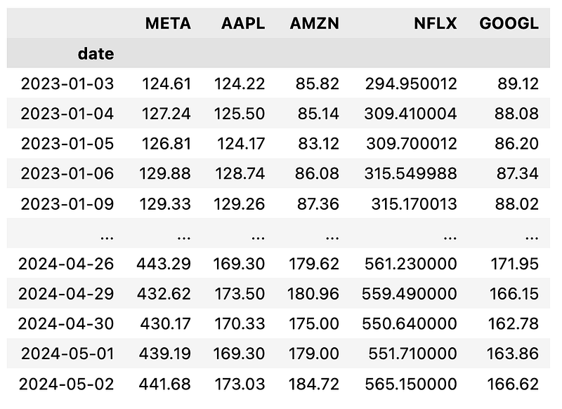
In the following code snippet, we download historical adjusted close prices for the FAANG companies from 2023 onward. The helper function downloads the prices for a single ticker, so we use a for loop to iterate over all of the selected stocks.

FAANG_TICKERS = ["META", "AAPL", "AMZN", "NFLX", "GOOGL"]
START_DATE = "2023-01-01"

def get_adj_close_price(symbol, start_date):
    hist_price_url = f"https://financialmodelingprep.com/api/v3/historical-price-full/{symbol}?from={start_date}&apikey={FMP_API_KEY}"
    r_json = requests.get(hist_price_url).json()
    df = pd.DataFrame(r_json["historical"]).set_index("date").sort_index()
    df.index = pd.to_datetime(df.index)
    return df[["adjClose"]].rename(columns={"adjClose": symbol})

price_df_list = []
for ticker in FAANG_TICKERS:
    price_df_list.append(get_adj_close_price(ticker, START_DATE))
prices_df = price_df_list[0].join(price_df_list[1:])
prices_df

Executing the code snippet returns the following DataFrame.

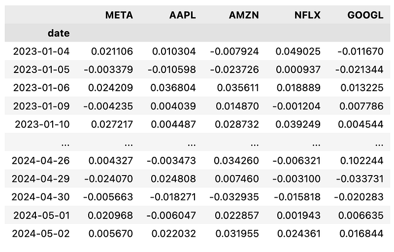
We still need to do one more thing: calculate returns from the prices. To do that, we will use the pct_change method of a pandas DataFrame.

returns_df = prices_df.pct_change().dropna()
returns_df

Portfolio optimization

Having prepared the data, we can proceed to finding the asset allocation for our portfolio. In the first example, we would like to find a portfolio that minimizes the risk (volatility). To do that, we need to complete the following three steps:

1. Calculate the expected returns for each asset (average returns over the selected time period) and the covariance matrix of the returns. We also annualize these values by multiplying them by the average number of trading days in a year (252).
2. Define a loss function. In this case, we would like to minimize the volatility. So, we need to define a function that calculates the portfolio volatility using the portfolio allocation (the value that we are trying to find) and the covariance matrix.
3. Run an optimization routine to find the allocation that minimizes the loss function. We will do that using scipy’s minimize function.

The following snippet contains steps 1 and 2:

# Calculate the annualized expected returns and the covariance matrix
avg_returns = returns_df.mean() * 252
cov_mat = returns_df.cov() * 252

# Define the function to find the portfolio volatility using the weights and the covariance matrix
def get_portfolio_volatility(weights, cov_mat):
    return np.sqrt(np.dot(weights.T, np.dot(cov_mat, weights)))

Then, we proceed to step 3:

# Define the number of assets
n_assets = len(avg_returns)

# Define the bounds - the weights can be between 0 and 1
bounds = tuple((0, 1) for asset in range(n_assets))

# Define the initial guess - the equally weighted portfolio
initial_guess = n_assets * [1.0 / n_assets]

# Define the constraint - all weights must add up to 1
constr = {"type": "eq", "fun": lambda x: np.sum(x) - 1}

# Find the minimum volatility portfolio
min_vol_portf = sco.minimize(
    get_portfolio_volatility,
    x0=initial_guess,
    args=cov_mat,
    method="SLSQP",
    constraints=constr,
    bounds=bounds,
)

This step is a bit more complex, as we had to prepare some additional inputs for the optimization routine:

• the bounds: we restrict the portfolio weights to values between 0 and 1, meaning there is no short selling.
• the initial guess: we use an equally-weighted portfolio as the initial guess. The optimization routine will start from that point. We can choose any values here, but 1/n weights are a reasonable first guess.
• the constraints: we also define some constraints that the weights must follow. In this case, we specify that the sum of all the weights must be equal to 100%, so we invest all of our capital.

After defining these, we run the optimization routine using the minimize function and get_portfolio_volatility as the loss function. After doing that, we can access the portfolio weights using the following snippet:

# Store the portfolio weights
min_vol_portf_weights = pd.Series(min_vol_portf.x, index=avg_returns.index).round(2)
min_vol_portf_weights

Using the historical data, we have identified the following portfolio as the one that minimizes volatility:

META     0.00
AAPL     0.74
AMZN     0.11
NFLX     0.07
GOOGL    0.08

Lastly, we can access the value of the function that we were minimizing (portfolio volatility) using the fun attribute: min_vol_portf.fun.

For the second example, let’s find a portfolio that maximizes the Sharpe ratio. As the general procedure has the very same steps, we just need to slightly adjust the code we have already prepared.

First, we need to define a new loss function. As we want to maximize the Sharpe ratio and the minimize function does the opposite, we define a function that calculates the negative Sharpe ratio.

def get_neg_sharpe_ratio(weights, avg_rtns, cov_mat, rf_rate):
    portf_returns = np.sum(avg_rtns * weights)
    portf_volatility = np.sqrt(np.dot(weights.T, np.dot(cov_mat, weights)))
    portf_sharpe_ratio = (portf_returns - rf_rate) / portf_volatility
    return -portf_sharpe_ratio

As you can see in the code, the function uses the portfolio weights, expected returns, the covariance matrix, and the risk-free rate. That is also why we need to provide the last three as arguments for the optimization routine. For simplicity (and to keep things realistic), let’s assume a risk-free rate of 0%.

RF_RATE = 0
args = (avg_returns, cov_mat, RF_RATE)

max_sharpe_portf = sco.minimize(
    get_neg_sharpe_ratio,
    x0=initial_guess,
    args=args,
    method="SLSQP",
    bounds=bounds,
    constraints=constr,
)

# Store the portfolio weights
max_sharpe_portf_weights = pd.Series(max_sharpe_portf.x, index=avg_returns.index).round(2)
max_sharpe_portf_weights

Using our optimization routine, we have identified the following weights as the ones that maximize the Sharpe ratio:

META     0.50
AAPL     0.00
AMZN     0.17
NFLX     0.21
GOOGL    0.11

We can also run max_sharpe_portf.fun to see that the value of the loss function after running the routine is -2.6415.

Evaluating the portfolios

In my previous article, I showed how to use quantstats to quickly evaluate the performance of trading strategies. We can also use that library to evaluate the performance of our portfolios!

To do so, we first need to calculate the portfolio returns. We can obtain those by multiplying the asset returns by the portfolio weights. Then, we calculate the performance metrics using quantstats. As the benchmark, we chose the S&P 500.

min_vol_portf_returns = returns_df.dot(min_vol_portf_weights)
qs.reports.metrics(min_vol_portf_returns, benchmark="SPY", mode="basic", rf=0)

                    Benchmark (SPY)    Strategy
------------------  -----------------  ----------
Start Period        2023-01-04         2023-01-04
End Period          2024-05-02         2024-05-02
Risk-Free Rate      0.0%               0.0%
Time in Market      100.0%             100.0%

Cumulative Return   31.6%              53.66%
CAGR﹪              15.37%             25.06%

Sharpe              1.68               1.75
Prob. Sharpe Ratio  97.32%             97.87%
Sortino             2.57               2.73
Sortino/√2          1.82               1.93
Omega               1.33               1.33

We only printed a few selected metrics for brevity’s sake. As you know by now, the tearsheet contains much more information, and I encourage you to take a look at it yourself and to generate some plots as well!

Finally, let’s also examine the performance metrics for the portfolio that maximizes the Sharpe ratio:

max_sharpe_portf_returns = returns_df.dot(max_sharpe_portf_weights)
qs.reports.metrics(max_sharpe_portf_returns, benchmark="SPY", mode="basic", rf=0)

                    Benchmark (SPY)    Strategy
------------------  -----------------  ----------
Start Period        2023-01-04         2023-01-04
End Period          2024-05-02         2024-05-02
Risk-Free Rate      0.0%               0.0%
Time in Market      100.0%             100.0%

Cumulative Return   31.6%              167.27%
CAGR﹪              15.37%             66.84%

Sharpe              1.68               2.6
Prob. Sharpe Ratio  97.32%             99.96%
Sortino             2.57               4.85
Sortino/√2          1.82               3.43
Omega               1.6                1.6

We can see that the value of the Sharpe ratio is equal to the one we received as the result of the optimization routine.

Wrapping up

In this article, we explored mean-variance optimization to find portfolio weights that result in portfolios with either minimum volatility or maximum Sharpe ratio. To do that, we used scipy to carry out the optimization routine. However, we could also use specialized libraries to do all the heavy lifting for us. We will explore an example of such a library next time!

If you are interested in learning more about using Python within the financial context, I’ve published a book that you might find interesting. In Python for Finance Cookbook, I present over 80 examples of using modern Python libraries for tasks such as time series forecasting, asset allocation, backtesting trading strategies, and much more. You can find more information about the book here and in this article.

You can find the code used in this article in this repository. As always, any constructive feedback is more than welcome. You can reach out to me on LinkedIn, Twitter, or in the comments.

Until next time 👋

You might also be interested in one of the following: