
Portfolio Optimization with Python: Mean-Variance Optimization (MVO) and Markowitz’s Efficient Frontier
In the realm of finance, constructing an optimal investment portfolio that maximizes returns while minimizing risk has always been a primary goal for investors. The process of achieving this balance between risk and return, known as portfolio optimization, has been extensively studied and refined over the years. Among the most prominent approaches to portfolio optimization, Mean-Variance Optimization (MVO) pioneered by Harry Markowitz stands as a cornerstone in modern portfolio theory. Its revolutionary concept of diversification opened the door to a more systematic and mathematical way of managing investments.
In this article, we delve into the world of portfolio optimization using Python, exploring the fundamental principles of Mean-Variance Optimization and its ability to shape an investor’s decision-making process. Additionally, we will explore Markowitz’s Efficient Frontier, a crucial concept that identifies the optimal combination of assets in a portfolio. Whether you are a seasoned investor or a Python enthusiast looking to deepen your knowledge of finance, this journey through the intricacies of portfolio optimization will provide valuable insights and practical tools for building well-balanced investment strategies. Let’s embark on this exciting exploration of financial analysis, programming, and modern portfolio theory.
Importance of portfolio optimization

Portfolio optimization is a crucial concept in managing investments, especially when dealing with a diverse range of assets, such as the top 100 companies listed on the NASDAQ. The significance of portfolio optimization lies in its ability to help investors achieve their financial goals while managing risk effectively.
Here are some key aspects of its importance:
- Diversification: Portfolio optimization encourages diversification, spreading investments across different assets and sectors. By holding a variety of stocks from the top 100 NASDAQ companies, investors can reduce the impact of poor performance in any single stock on their overall portfolio. Diversification helps lower overall risk and potentially enhances returns.
- Risk Management: Risk is an inherent part of investing. Through portfolio optimization, investors can analyze the risk-return trade-offs of different assets and construct portfolios that align with their risk tolerance. It allows investors to strike a balance between seeking higher returns and preserving capital during market downturns.
- Maximizing Returns: The ultimate goal of investing is to maximize returns. Portfolio optimization involves strategic allocation of assets to achieve the best possible returns within the given risk parameters. By selecting a combination of assets with varying risk profiles and expected returns, investors can aim to optimize their portfolio’s overall performance.
- Capital Preservation: Preservation of capital is equally important as generating returns, especially for risk-averse investors. Portfolio optimization enables the allocation of assets in a manner that ensures the capital is protected while still participating in potential growth opportunities.
- Efficient Frontier: Portfolio optimization helps identify the efficient frontier, which represents the set of portfolios with the highest expected return for a given level of risk or the lowest risk for a given level of return. Investors can use this concept to choose the most appropriate portfolio based on their risk appetite and return objectives.
- Rebalancing: Markets are dynamic, and asset values change over time, causing the portfolio’s asset allocation to deviate from the original plan. Portfolio optimization facilitates regular rebalancing to maintain the desired risk and return characteristics, ensuring that the portfolio stays aligned with the investor’s objectives.
- Long-Term Planning: Successful investing requires a long-term perspective. Portfolio optimization assists investors in creating a well-structured and diversified portfolio that aligns with their long-term financial goals, such as retirement planning or funding future expenses.
- Data-Driven Decision Making: Modern portfolio optimization techniques leverage sophisticated mathematical models and historical data to make informed investment decisions. By incorporating quantitative analysis, investors can minimize emotional biases and base their choices on empirical evidence.
In the context of the top 100 NASDAQ companies, portfolio optimization becomes particularly important due to the sheer number of investment options available. These companies represent a wide array of industries, risk profiles, and growth potentials. By employing portfolio optimization techniques, investors can navigate the complexities of this market and build portfolios that aim to deliver optimal returns while managing risk effectively.
Brief Overview of the Portfolio Models of Focus: Mean-Variance Optimization (MVO), Markowitz’s Efficient Frontier, and the Black-Litterman model.
- Mean-Variance Optimization (MVO)
Mean-Variance Optimization, developed by Nobel laureate Harry Markowitz, is a fundamental concept in modern portfolio theory. It aims to construct an optimal investment portfolio by balancing the trade-off between expected returns and risk. MVO takes into account the historical returns and volatilities of individual assets and their correlations to create a diversified portfolio that maximizes returns for a given level of risk or minimizes risk for a target level of return. The main output of MVO is the Efficient Frontier, which represents a range of optimal portfolios with varying risk levels. However, MVO has limitations, such as sensitivity to input data and potential issues with assumptions, which led to the development of more sophisticated models like the Black-Litterman model.
2. Markowitz’s Efficient Frontier
Markowitz’s Efficient Frontier is a critical concept derived from MVO. It represents a graph that plots the various portfolios that offer the maximum expected return for each level of risk or the minimum risk for each level of expected return. Portfolios on the Efficient Frontier are considered efficient because they provide the highest expected returns for their given risk or the lowest risk for their expected returns. By identifying the Efficient Frontier, investors can choose the optimal mix of assets that best suits their risk appetite and financial goals, offering a systematic approach to portfolio diversification.

In recent years, Python has emerged as one of the most popular and versatile programming languages for data analysis, financial modeling, and portfolio optimization in the realm of finance. Python’s relevance as the programming language for portfolio optimization analysis of the top 100 NASDAQ companies lies in its robust data analysis capabilities and a vast ecosystem of specialized libraries. These qualities make Python an ideal choice for efficiently handling and processing financial data, implementing sophisticated models, and generating insightful visualizations. Here are some key reasons why Python stands out for this analysis:
1. Rich Ecosystem of Libraries: Python boasts a vast ecosystem of powerful libraries and frameworks specifically designed for data manipulation, numerical computing, and financial analysis. Libraries like NumPy, Pandas, and SciPy provide robust data structures and efficient mathematical functions, enabling the smooth handling of financial data and complex computations.
2. Data Visualization Capabilities: Python offers a variety of visualization libraries, including Matplotlib, Seaborn, and Plotly, which facilitate the creation of insightful charts and graphs to visualize portfolio performance, asset allocations, and risk profiles. These visualizations aid in making data-driven investment decisions and communicating results effectively.
3. Accessibility and Readability: Python’s clean and readable syntax makes it accessible to both finance professionals and programmers. Its simplicity and expressiveness allow for faster development and easier collaboration, even for individuals with limited coding experience.
4. Active Community Support: Python’s finance and data science communities are exceptionally active and continuously contribute to the development of libraries, tools, and tutorials. This active support fosters knowledge sharing and quick resolution of issues, ensuring that developers have access to the latest advancements and best practices.
5. Integration with Web Technologies: Python’s ability to integrate seamlessly with web technologies makes it suitable for building interactive financial dashboards, web applications, and APIs. This feature is especially valuable for investors and fund managers who wish to monitor and manage their portfolios in real time.
6. Machine Learning Capabilities: With the rise of machine learning in finance, Python’s popular machine learning libraries like Scikit-learn and TensorFlow enable investors to apply advanced techniques for predicting market trends, risk analysis, and portfolio optimization strategies.
7. Open-Source and Cost-Effective: Python is open-source, making it freely available for anyone to use and modify. This cost-effective aspect is particularly appealing to financial professionals and researchers working on various budget constraints.
In conclusion, the combination of Python’s rich libraries, user-friendly syntax, strong community support, and machine-learning capabilities positions it as an ideal choice for implementing portfolio optimization. Its versatility empowers finance professionals to analyze complex data, construct efficient portfolios, and gain valuable insights that drive smarter investment decisions. As a result, Python has become an indispensable tool in the finance industry, revolutionizing the way portfolios are constructed, analyzed, and managed.
An overview of the NASDAQ stock exchange and its significance in the technology and growth sectors

The NASDAQ (National Association of Securities Dealers Automated Quotations) is a prominent stock exchange in the United States, known for its focus on technology and growth-oriented companies. Established in 1971, NASDAQ was the world’s first electronic stock market, introducing automated trading systems and electronic quotation systems, which revolutionized the way securities were bought and sold.
NASDAQ operates as a fully electronic exchange, meaning that all trading occurs through computer networks without a physical trading floor. It is a dealer’s market, where market makers facilitate trading by providing bid and ask prices for various securities, including stocks, options, and exchange-traded funds (ETFs).
Significance in Technology:
NASDAQ’s significance in the technology sector stems from its reputation as a preferred listing venue for technology-based companies. Many of the world’s leading technology giants, including Apple, Microsoft, Amazon, Google (Alphabet), and Facebook, are listed on NASDAQ. This concentration of tech companies on the exchange has earned it the nickname “The Silicon Valley of Capital” and solidified its position as a hub for innovative and high-growth technology firms.
NASDAQ’s technology-oriented focus makes it an attractive platform for startups and emerging tech companies seeking access to public capital. The exchange’s ability to accommodate companies with high growth potential has contributed to its reputation as the go-to-market for tech IPOs (Initial Public Offerings).
Significance in Growth Sectors:
NASDAQ’s emphasis on growth is evident through its selection of companies. The exchange has a greater representation of growth-oriented industries, such as technology, biotechnology, pharmaceuticals, clean energy, and consumer discretionary sectors. These industries are known for their potential for rapid expansion and substantial market opportunities.
The listing requirements and governance standards set by NASDAQ are often more lenient compared to traditional stock exchanges like the New York Stock Exchange (NYSE). This makes it an attractive option for smaller companies and startups that do not meet the stringent criteria of other exchanges.
Additionally, NASDAQ’s technology-driven and innovative nature appeals to companies with disruptive business models and novel products, further contributing to its reputation as a platform for growth-oriented firms.
Selection Criteria for the Top 100 NASDAQ Companies
The Nasdaq-100 is a stock market index that tracks the performance of the 100 largest non-financial companies listed on the Nasdaq stock exchange. The index is reconstituted annually in December, and the selection criteria are as follows:
- Market Capitalization: Market capitalization refers to the total value of a company’s outstanding shares of stock. It is one of the primary factors used to determine a company’s size and is calculated by multiplying the current stock price by the total number of outstanding shares. Companies with higher market capitalizations are generally considered larger and more established, making them attractive investment options for many investors. In the context of the top 100 NASDAQ companies, those with the highest market capitalizations are more likely to be included due to their significance in the market and overall economy.
- Trading Volume: Trading volume represents the total number of shares traded in a company’s stock over a given period, typically a day or a month. It is an essential criterion because it reflects the liquidity and interest in a company’s stock. Higher trading volumes generally indicate more active investor interest, making it easier to buy or sell shares without significantly impacting the stock’s price. Companies with substantial trading volumes are often more attractive to investors seeking easy access to the market and reduced bid-ask spreads.
- Industry Representation: The NASDAQ includes companies from various industries, including technology, healthcare, finance, consumer goods, and more. Industry representation is a critical factor in ensuring diversification within the top 100 companies. A balanced representation across different sectors helps spread the investment risk and reduces the impact of industry-specific challenges on the overall market performance.
- Financial Performance and Stability: While market capitalization, trading volume, and industry representation play significant roles, the financial performance and stability of a company are equally essential. Companies with strong earnings growth, revenue generation, and profitability are more likely to be considered for inclusion in the top 100 NASDAQ companies. Moreover, financial stability, low debt levels, and positive cash flow are factors that investors often prioritize.
- Compliance with NASDAQ Listing Requirements: The NASDAQ Stock Market has specific listing requirements that companies must meet to be listed on the exchange. These requirements include criteria related to the number of publicly traded shares, minimum bid price, financial standards, and corporate governance rules. Companies must maintain compliance with these listing requirements to remain on the exchange and be eligible for inclusion in the top 100 companies.
Here is a table that summarizes the selection criteria for the Nasdaq-100:
The Challenges and Opportunities Associated with The Top 100 Nasdaq Stocks
Constructing portfolios from a dynamic and diverse set of companies, such as the top 100 NASDAQ companies, presents both challenges and opportunities for investors. These challenges and opportunities arise due to the unique characteristics of the companies involved, the fast-paced nature of the technology sector, and the constantly evolving market dynamics. Let’s explore them in detail:
Challenges
- Volatility and Risk Management: Technology companies, especially startups and growth-oriented firms, tend to exhibit higher volatility compared to established companies in other sectors. This increased volatility can pose challenges in managing risk, as the portfolio’s overall risk level may become elevated. Risk management strategies need to be carefully employed to ensure that the portfolio remains aligned with the investor’s risk tolerance.
- Information Asymmetry: Startups and emerging tech companies may lack a substantial track record, making it challenging to assess their true growth potential accurately. Investors may face information asymmetry, where they have limited access to reliable data, financials, and performance metrics, complicating the decision-making process.
- Market Sentiment and Hype: The technology sector is highly influenced by market sentiment and can experience significant price swings based on news, speculation, or even social media trends. This can lead to market exuberance or irrational pessimism, impacting the overall performance of the portfolio.
- Sector Concentration Risk: The top 100 NASDAQ companies may represent a substantial concentration in specific sectors, such as technology and biotechnology. Overexposure to a particular sector can increase the vulnerability of the portfolio to adverse events affecting that sector.
- Liquidity Concerns: Smaller tech companies or those recently listed may have lower liquidity compared to large-cap stocks. This can impact the ease of buying or selling positions in the portfolio, potentially resulting in higher transaction costs and difficulties in executing trades at desired prices.
Opportunities
- High Growth Potential: The dynamic and diverse set of companies in the technology sector offers significant growth potential. Investing in well-selected tech companies can provide an opportunity for substantial capital appreciation, outperforming broader market indices during periods of robust growth.
- Innovation and Disruption: Technology companies are often at the forefront of innovation and disruptive technologies. Investors can leverage opportunities arising from transformative breakthroughs and groundbreaking products that reshape industries.
- Diversification Benefits: The NASDAQ’s diverse set of companies encompass various sectors, including technology, healthcare, consumer goods, and more. This diversity allows investors to build portfolios that span multiple industries, reducing the impact of adverse events affecting any single sector.
- Early-Stage Investment Access: NASDAQ’s appeal to startups and growing companies provides investors with access to companies in their early stages, which may become significant players in the future. Early investment in potential market leaders can yield substantial returns.
- Real-Time Performance Monitoring: The technology-driven nature of the NASDAQ enables investors to access real-time market data, news, and updates on their portfolio holdings. This facilitates timely decision-making and adjustments to align with changing market conditions.
Mean-Variance Optimization (MVO) for Top 100 NASDAQ
In constructing efficient portfolios for NASDAQ companies, mean-variance optimization can be used to select a combination of stocks that maximizes expected return while minimizing risk. The process involves selecting stocks with low correlation to each other so that diversification can be achieved. MVO aims to find the optimal allocation of assets in a portfolio that maximizes expected returns for a given level of risk or minimizes risk for a target level of expected returns. Here’s an overview of the foundations of MVO and its relevance in constructing efficient portfolios for the selected NASDAQ companies.
Foundations of Mean-Variance Optimization:
- Expected Return: The first step in MVO is estimating the expected returns of individual assets in the portfolio. The expected return is the mean or average return that investors anticipate based on historical data, fundamental analysis, or other forecasting methods.
- Risk (Variance or Standard Deviation): Risk is quantified as the variance or standard deviation of returns. In MVO, risk represents the volatility or uncertainty associated with an asset’s future performance. Assets with higher variance or standard deviation are considered riskier because their returns tend to fluctuate more.
- Covariance: MVO takes into account the covariance between asset returns. Covariance measures how two assets move together. Positive covariance implies that the assets tend to move in the same direction, while negative covariance means they move in opposite directions. A higher covariance between assets increases the overall portfolio risk.
- Efficient Frontier: The core idea of MVO is to find the optimal mix of assets that lie on the efficient frontier. The efficient frontier represents a set of portfolios with the maximum expected return for a given level of risk or the minimum risk for a given level of expected return. It is a curved boundary that depicts the best possible risk-return trade-offs for various asset combinations.
Relevance in Constructing Efficient Portfolios for NASDAQ Companies:
- Diversification: The top 100 NASDAQ companies span various industries, sizes, and risk profiles. By applying MVO, investors can determine the ideal allocation of assets to achieve diversification and spread risk across different companies and sectors. This diversification can help reduce the overall portfolio risk without significantly sacrificing expected returns.
- Risk Management: MVO allows investors to set risk constraints based on their risk tolerance levels. For example, an investor might want to limit the portfolio’s maximum risk or target a specific level of risk. MVO helps identify the mix of NASDAQ companies that align with these risk parameters.
- Return Maximization: MVO assists investors in constructing portfolios that aim to achieve the highest possible expected return for a given level of risk. By carefully selecting assets with strong growth potential and favorable risk-return characteristics, the investor can maximize returns while managing risk effectively.
- Rebalancing: The dynamic nature of financial markets requires regular portfolio rebalancing. MVO provides a quantitative framework to analyze the changing risk and return profiles of assets and helps investors determine when and how to rebalance their portfolios to stay aligned with their investment objectives.
- Quantitative Decision-Making: MVO leverages mathematical optimization techniques to objectively identify optimal portfolios based on historical data and projected returns. This data-driven approach helps investors minimize emotional biases and make well-informed decisions when constructing their portfolios.
Usage of Top 100 Nasdaq Stocks Historical Data
Historical data on stock prices and returns are essential for various financial analyses, including computing mean returns, standard deviations, and correlation coefficients. These statistical measures provide valuable insights into the performance and risk characteristics of individual stocks and their relationships with other assets in a portfolio. Here’s how historical data is used to compute these metrics:
- Mean Return (Expected Return):
Mean return, also known as the expected return, is the average return of an asset over a specific period, typically calculated on a daily, monthly, or annual basis. To compute the mean return, follow these steps:
- Collect Historical Prices: Gather historical price data of the stock for the desired time period, represented as a time series of daily, monthly, or annual prices.
- Calculate Daily Returns: Calculate the daily returns of the stock by using the formula: Daily Return (t) = (Price (t) — Price (t-1)) / Price (t-1)
- Compute Mean Return: Calculate the mean of the daily returns to obtain the average return over the chosen period. The mean return is typically annualized by multiplying it by the number of periods in a year (e.g., 252 trading days for daily returns).
2. Standard Deviation (Risk):
Standard deviation measures the dispersion or variability of a stock’s returns around its mean return. A higher standard deviation indicates higher volatility or risk. To compute the standard deviation, follow these steps:
- Use the Historical Daily Returns: Utilize the same daily return data calculated earlier.
- Calculate the Mean Return: Compute the mean return of the stock over the chosen period.
- Calculate Deviations: For each daily return, subtract the mean return from the actual daily return to obtain the deviation from the mean.
- Square the Deviations: Square each deviation to avoid negative values.
- Calculate the Variance: Sum up all squared deviations and divide by the number of periods minus one (to compute the sample variance) or use the number of periods (if it represents the entire population).
- Compute the Standard Deviation: Take the square root of the variance to get the standard deviation.
3. Correlation Coefficients:
Correlation coefficients measure the degree of linear relationship between the returns of two assets. It ranges from -1 to +1, with -1 indicating a perfect negative correlation, +1 indicating a perfect positive correlation, and 0 indicating no linear correlation. To compute the correlation coefficient, follow these steps:
- Collect Historical Daily Returns: Gather the historical daily return data for both stocks you want to analyze.
- Calculate the Mean Returns: Compute the mean returns for both stocks.
- Calculate Deviations from the Mean: For each day, find the deviation from the mean for both stocks’ returns.
- Calculate Covariance: Multiply the deviations of each day for both stocks and sum them up over the chosen period. Then divide by the number of periods minus one (sample covariance) or use the number of periods (population covariance).
- Compute the Correlation Coefficient: Divide the covariance by the product of the standard deviations of both stocks to get the correlation coefficient.
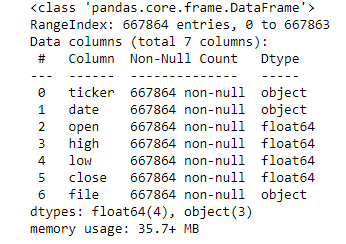
Implementing Mean-Variance Optimization (MVO) in Python involves using numerical optimization techniques to find the optimal allocation of assets in a portfolio that maximizes returns for a given level of risk or minimizes risk for a target level of returns. We’ll use the numpy library for numerical computations and the scipy library for optimization. Additionally, we'll use historical stock price data to compute mean returns, covariance matrix, and standard deviations. To demonstrate, let's assume we have historical price data for three NASDAQ companies: AAPL (Apple Inc.), MSFT (Microsoft Corporation), and AMZN (Amazon.com Inc.).
First, make sure you have the necessary libraries installed. You can install them using pip:
pip install numpy scipy pandas
We have the following historical data:
Let’s us do a data exploration and clean up by:
- Check for Missing and Duplicate entries in our Dataframe:
null_val_sums1 = df1.isnull().sum()
duplicate1 = data[df1.duplicated()].shape[0]
pd.DataFrame({"Column": null_val_sums1.index, "Number of Null/MIssing Values": null_val_sums1.values,
              "Number of Duplicate Values":duplicate1, "Proportion/Count": null_val_sums1.values / len(df1), "Data Type": df1.dtypes })
2. Convert dates to datetime format.
df1['date'] = pd.to_datetime(df1['date'])3. Dropping unnecessary columns
df1.drop(['file'], axis=1, inplace=True)4. Feature Engineering: Adding Potential useful features
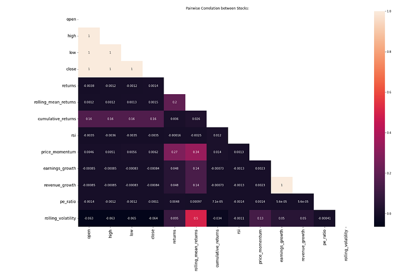
df1['returns'] = df1.groupby('ticker')['close'].pct_change()
df1['returns'] = df1.groupby('ticker')['returns'].fillna(df1['returns'].mean())

df1['cumulative_returns'] = df1.groupby('ticker')['returns'].cumsum()

window = 14
delta = df1.groupby('ticker')['close'].diff()
gain = delta.where(delta > 0, 0)
loss = -delta.where(delta < 0, 0)
average_gain = gain.rolling(window).mean().reset_index(0, drop=True)
average_loss = loss.rolling(window).mean().reset_index(0, drop=True)
rs = average_gain / average_loss
df1['rsi'] = 100 - (100 / (1 + rs))
df1['rsi'] = df1.groupby('ticker')['rsi'].fillna(df1['rsi'].mean())


lookback_period = 10
df1['price_momentum'] = df1.groupby('ticker')['close'].pct_change(lookback_period)
df1['price_momentum'] = df1.groupby('ticker')['price_momentum'].fillna(df1['price_momentum'].mean())

# Calculate earnings_growth, revenue_growth, and pe_ratio
df1['earnings_growth'] = df1.groupby('ticker')['returns'].pct_change()
df1['revenue_growth'] = df1.groupby('ticker')['returns'].pct_change()
df1['pe_ratio'] = df1['close'] / df1['returns']
df1.replace([np.inf, -np.inf], np.nan, inplace=True)
df1['earnings_growth'] = df1.groupby('ticker')['earnings_growth'].fillna(df1['earnings_growth'].mean())
df1['revenue_growth'] = df1.groupby('ticker')['revenue_growth'].fillna(df1['revenue_growth'].mean())
df1['pe_ratio'] = df1.groupby('ticker')['pe_ratio'].fillna(df1['pe_ratio'].mean())

df1['rolling_volatility'] = df1.groupby('ticker')['returns'].rolling(window=30, min_periods=1).std().reset_index(0, drop=True)
df1['rolling_volatility'] = df1.groupby('ticker')['rolling_volatility'].fillna(df1['rolling_volatility'].mean())
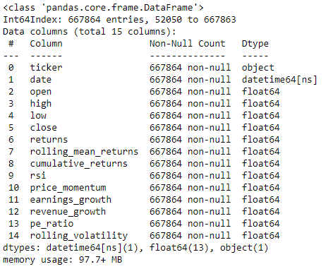
Now we have the following data:
Then we estimate the expected returns for each asset in your universe. We can use historical returns, fundamental analysis, or other methods to estimate future returns.
expected_returns = df1.groupby('ticker')['returns'].mean()After we then determine the weighting scheme for our portfolio. Common methods include equal weighting, market capitalization weighting, or using optimization techniques to determine the optimal weights.
- Equal weighting
num_assets = len(df1['ticker'].unique())
weights = pd.Series(1/num_assets, index=df1['ticker'].unique())- mean-variance optimization approach
covariance_matrix = df1.pivot_table(index='date', columns='ticker', values='returns', aggfunc=np.mean).cov()
expected_returns = df1.groupby('ticker')['returns'].mean()
# Number of assets
n_assets = len(expected_returns)

# Define the optimization variables
weights = cp.Variable(n_assets)
target_return = cp.Parameter()

# Define constraints
constraints = [
    cp.sum(weights) == 1,
    weights >= 0
]

# Define the portfolio risk
portfolio_risk = cp.quad_form(weights @ covariance_matrix.values, np.eye(n_assets))

# Define the objective (minimize portfolio risk)
objective = cp.Minimize(portfolio_risk)

# Define the problem
problem = cp.Problem(objective, constraints)

# Solve the problem
problem.solve()

# Get the optimal weights
optimal_weights = weights.value

# Print the optimal weights
print("Optimal Weights:")
print(optimal_weights)- Sharpe ratio optimization
covariance_matrix = df1.pivot_table(index='date', columns='ticker', values='returns', aggfunc=np.mean).cov()
expected_returns = df1.groupby('ticker')['returns'].mean()
def negative_sharpe_ratio(weights):
    portfolio_return = np.dot(weights, expected_returns)
    portfolio_variance = np.dot(weights, np.dot(covariance_matrix, weights))
    sharpe_ratio = (portfolio_return - risk_free_rate) / np.sqrt(portfolio_variance)
    return -sharpe_ratio

# Define the equality constraint
constraint = {'type': 'eq', 'fun': lambda x: np.sum(x) - 1}

# Define the bounds on the variables
bounds = [(0, 1) for _ in range(n_assets)]

# Set an initial guess for the weights (equal weights)
initial_weights = np.ones(n_assets) / n_assets

# Use the SLSQP optimization algorithm to find the optimal weights
result = minimize(negative_sharpe_ratio, initial_weights, method='SLSQP', constraints=constraint, bounds=bounds)
optimal_weights = result.x

# Print the weights
print("Optimal Weights:")
for i, weight in enumerate(optimal_weights):
    print(f"Stock {i+1}: {weight}")
Next, let’s create a simple Python script to implement MVO:
import numpy as np
import pandas as pd
from scipy.optimize import minimize

returns_data = {
    'AAPL': [0.001, 0.002, -0.003, 0.004, 0.001],
    'MSFT': [0.002, 0.001, 0.005, 0.003, -0.002],
    'AMZN': [0.003, 0.004, 0.002, 0.001, 0.006]
}

returns_df = pd.DataFrame(returns_data)

def mean_variance_optimization(returns_df):
    # Calculate mean returns and covariance matrix
    mean_returns = returns_df.mean()
    cov_matrix = returns_df.cov()

    num_assets = len(returns_df.columns)

    # Function to minimize - negative portfolio returns (to maximize returns)
    def negative_portfolio_returns(weights):
        return -np.sum(mean_returns * weights)

    weight_sum_constraint = {'type': 'eq', 'fun': lambda weights: np.sum(weights) - 1}

    bounds = tuple((0, 1) for _ in range(num_assets))

    initial_weights = np.ones(num_assets) / num_assets

    # Perform MVO optimization
    result = minimize(negative_portfolio_returns, initial_weights, method='SLSQP', bounds=bounds, constraints=[weight_sum_constraint])

    return result.x

def main():
    optimized_weights = mean_variance_optimization(returns_df)
    print("Optimal Weights:", optimized_weights)

if __name__ == "__main__":
    main()
In this example, we calculate the mean returns and covariance matrix from the historical daily return data of the three companies. We then define the objective function to minimize (negative portfolio returns) and set the constraint that the weights must sum to 1. The minimize function from scipy.optimize is used to perform the optimization using the Sequential Least SQuares Programming (SLSQP) algorithm.
The output will provide the optimal weights for the three assets in the portfolio that maximize returns given the historical data and risk parameters.
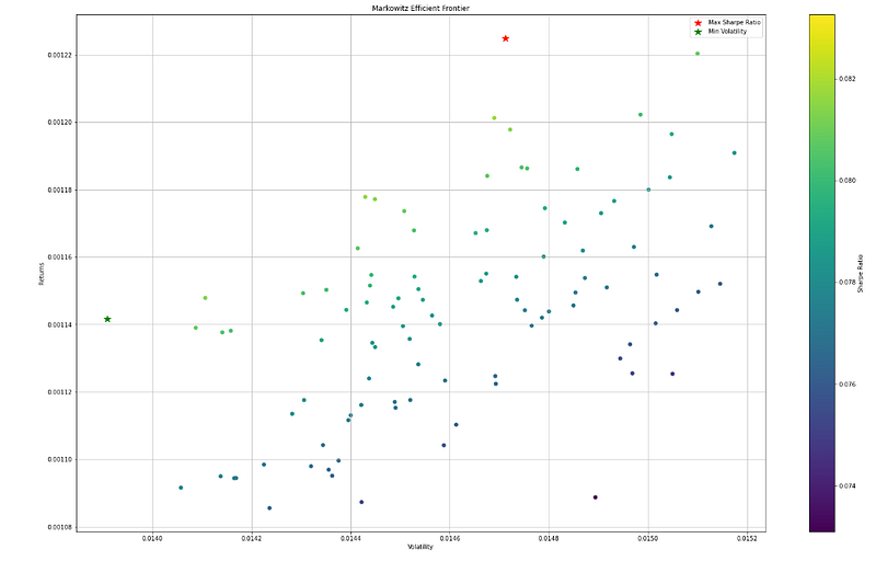
Exploring Markowitz’s Efficient Frontier
When applying Markowitz’s Efficient Frontier to the top 100 NASDAQ companies, several key aspects come into play. Firstly, diversification is emphasized as a means of managing risk. The top 100 NASDAQ companies span various industries, each with its unique set of risks and growth prospects. By diversifying across different sectors and companies, investors can reduce the impact of poor performance in any single stock on the overall portfolio, potentially enhancing returns while mitigating risk.
Moreover, the Efficient Frontier helps investors identify the optimal portfolio that aligns with their risk preferences. It enables them to visualize the risk-return trade-offs, allowing them to choose portfolios with risk levels that suit their comfort level while still aiming for reasonable returns. Furthermore, the concept aids in selecting portfolios that offer the highest expected returns for a given level of risk. By carefully selecting companies with strong growth potential, favorable financial performance, and positive market outlooks, investors can construct portfolios that seek to maximize returns within their risk constraints.
The Efficient Frontier also allows investors to construct portfolios that are efficient in terms of risk and return. By combining assets with different correlations, investors can achieve superior risk diversification and optimize the portfolio’s overall performance. Markowitz’s model provides a mathematical approach to determining the optimal asset allocation. Additionally, the concept assists in identifying when and how to rebalance portfolios as market conditions change. This ensures that investors maintain their position on the optimal risk-return curve and adapt to evolving market dynamics. Let’s illustrate how the Efficient Frontier works and how it enables investors to make informed decisions:
Step 1: Portfolio Combinations
The Efficient Frontier is constructed by combining different proportions of assets in a portfolio. For example, suppose an investor is considering a portfolio comprising two assets: Company A and Company B. By varying the allocation between the two assets, different portfolios are formed. Each portfolio is represented by a point on a graph, where the x-axis represents the portfolio’s risk (standard deviation), and the y-axis represents the portfolio’s return (expected mean).
Step 2: Risk-Return Trade-off
As the investor allocates more weight to one asset relative to the other, the portfolio’s risk and return change. Portfolios with a higher allocation to a riskier asset tend to have higher expected returns, but also higher risk. Conversely, portfolios with a higher allocation to a less risky asset tend to have lower expected returns but also lower risk. The Efficient Frontier is the boundary that encompasses all these portfolio combinations, representing the optimal risk-return combinations achievable with the given set of assets.
Step 3: Identifying the Optimal Portfolio
The highest point on the Efficient Frontier represents the portfolio with the maximum return for a given level of risk. This portfolio is known as the Tangency Portfolio or the Maximum Sharpe Ratio Portfolio. It offers the highest risk-adjusted return, meaning it provides the best return per unit of risk. This point is a crucial reference for investors, as it allows them to identify the portfolio that offers the most attractive risk-return trade-off.
Step 4: Informed Decision-Making
By analyzing the Efficient Frontier, investors can make informed decisions based on their risk appetite and financial goals. Here’s how the Efficient Frontier helps in decision-making:
- Risk Tolerance: Investors with a low-risk tolerance can choose portfolios located towards the left of the Efficient Frontier, representing lower risk profiles. On the other hand, those with a higher risk tolerance may opt for portfolios located further to the right, offering higher returns with more significant risk.
- Diversification Benefits: The Efficient Frontier showcases the benefits of diversification. By combining assets with low or negative correlations, investors can create portfolios that lie below the Efficient Frontier, meaning they achieve a higher return for a given level of risk compared to individual assets.
- Performance Evaluation: Investors can evaluate their current portfolio’s risk-return characteristics by comparing its position relative to the Efficient Frontier. If the portfolio lies below the Efficient Frontier, there is room for improvement through better asset allocation.
- Portfolio Optimization: The Efficient Frontier guides investors in constructing portfolios that align with their financial objectives. Investors can optimize their portfolios by choosing the asset allocation that lies on the Efficient Frontier or selecting the Tangency Portfolio for the best risk-adjusted return.
By understanding the trade-off between risk and return, investors can design well-balanced and efficient portfolios that align with their individual risk tolerance and investment objectives. The Efficient Frontier’s graphical representation simplifies the decision-making process, providing a clear visualization of the portfolio’s risk and return characteristics, ultimately leading to more prudent and informed investment choices.
Implementation of Solving Markowitz’s Efficient Frontier with constrained optimization method in Python
Calculating the Efficient Frontier
There are 2 inputs we must compute before finding the Efficient Frontier for our stocks: annualized rate of return and covariance matrix.
Annualized rate of return is calculated by multiplying the daily percentage change for all of the stocks with the number of business days each year (252).
#Calculate daily changes in the stocks' value
df2 = df1.pct_change()
#Remove nan values at the first row of df2. Create a new dataframe df
df=df2.iloc[1:len(df2.index),:]
# Calculate annualized average return for each stock. Annualized average return = Daily average return * 252 business days.
r = np.mean(df,axis=0)*252

# Create a covariance matrix
covar = df.cov()
Next, we should define some functions that we will use later in our calculation.
- Rate of return is the annualized rate of return for the whole portfolio.
- Volatility is the risk level, defined as the standard diviation of return.
- Sharpe ratio is risk efficiency; it assesses the return of an investment compared to its risk.
def ret(r,w):
    return r.dot(w)
# Risk level - or volatility
def vol(w,covar):
    return np.sqrt(np.dot(w,np.dot(w,covar)))
def sharpe (ret,vol):
    return ret/vol
The problem now is how to optimize our portfolio. Let’s say we want the lowest level of risk possible. Thus, we should find a portfolio with minimum volatility. It is a straightforward minimization problem. However, there are certain boundaries we must conform to:
- All weights must be between 0 and 1 (as we cannot buy a negative amount of stocks, and we cannot form a portfolio with more than 100% of 1 stock).
- The sum of weights of all stock must be 1.
Now, we should choose an algorithm to optimize our portfolio. Generalized Reduced Gradient Method is a feasible choice, but there are no libraries that have it. If you want to, you can read about this algorithm here, or try this code found on Github. Otherwise, we can explore some of the available choices in scipy.optimize. TheTrust-Region Constrained Algorithm (method=’trust-constr’) since it is suitable for multivariate scalar functions.
import numpy as np
from scipy.optimize import minimize, LinearConstraint, Bounds

num_assets = df2.shape[1]

# All weights must be between 0 and 1, so set 0 and 1 as the boundaries.
bounds = Bounds(0, 1)

# Set the constraint that the sum of weights equals 1.
constraint_matrix = np.ones((1, num_assets))
linear_constraint = LinearConstraint(constraint_matrix, [1], [1])

# Find a portfolio with the minimum risk.
# Create x0, the first guess at the values of each stock's weight.
initial_weights = np.ones(num_assets) / num_assets

# Define a function to calculate portfolio volatility (risk)
def portfolio_volatility(weights):
    return np.sqrt(np.dot(weights, np.dot(weights, covar)))

# Minimize the risk function using the 'trust-constr' method with linear constraint and bounds.
res = minimize(portfolio_volatility, initial_weights, method='trust-constr', constraints=linear_constraint, bounds=bounds)

# These are the weights of the stocks in the portfolio with the lowest level of risk possible.
w_min = res.x

# Set print options to show weights and risk with 2 decimal places
np.set_printoptions(suppress=True, precision=2)

# Print the optimal weights and corresponding return and risk
print("Optimal Weights:")
print(w_min)
print("Return: %.2f%%" % (ret(r, w_min) * 100), "Risk: %.3f" % portfolio_volatility(w_min))
What if we want to find a portfolio with the highest level of risk efficiency — that is, a portfolio that has the highest ratio of return/risk (Sharpe ratio)?
We can just use the same algorithm, with the same constraints, but this time, let’s optimize for the highest Sharpe ratio, which is a maximization problem. But…
“Maximization is for losers! We want to minimize!!”
Thus, we will find the minimum of 1/Sharpe_ratio instead.
# Create x0, the first guess at the values of each stock's weight.
initial_weights = np.ones(num_assets) / num_assets
# Define the function to calculate the Sharpe ratio (1/volatility)
def sharpe_ratio(weights):
portfolio_volatility = np.sqrt(np.dot(weights, np.dot(weights, covar)))
portfolio_return = np.dot(r, weights)
return -portfolio_return / portfolio_volatility # negative value for minimization
# Minimize the negative Sharpe ratio (to maximize Sharpe ratio) using 'trust-constr' method with constraints and bounds.
res_sharpe = minimize(sharpe_ratio, initial_weights, method='trust-constr', constraints=linear_constraint, bounds=bounds)
# These are the weights of the stocks in the portfolio with the highest Sharpe ratio.
w_sharpe = res_sharpe.x
# Set print options to show weights, return, and risk with 2 decimal places
np.set_printoptions(suppress=True, precision=2)
# Print the optimal weights and corresponding return and risk
print("Optimal Weights (Highest Sharpe Ratio):")
print(w_sharpe)
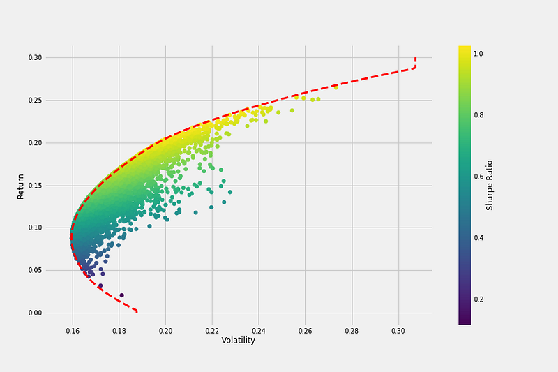
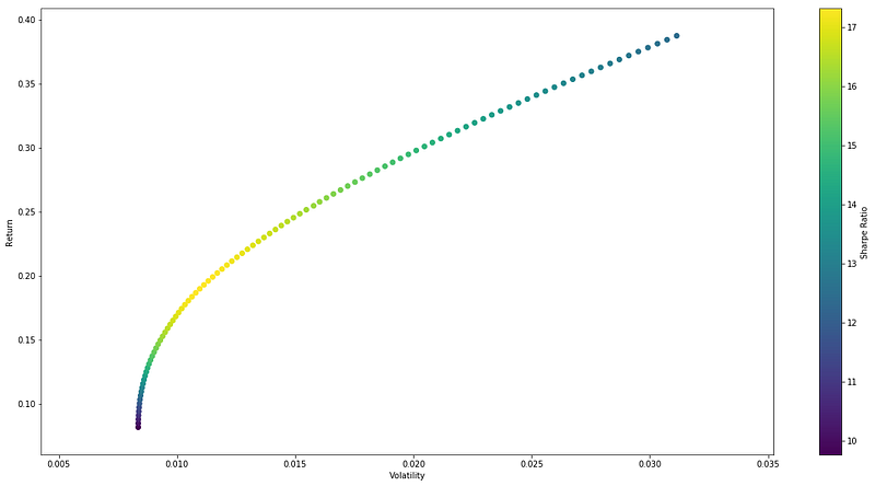
print("Return: %.2f%%" % (np.dot(r, w_sharpe) * 100), "Risk: %.3f" % np.sqrt(np.dot(w_sharpe, np.dot(w_sharpe, covar))))Great! What if we wish to depict the Efficient Frontier at this point? simply to check out the appearance?
Since we had determined the highest return for the lowest amount of risk, it is simple to begin there and gradually progress up the return axis, by, say, 100 points. The degree of risk is then optimized (minimized). Of course, with a minor modification, we can still apply the same approach.
# Initialize an array to store all the portfolio weights
all_weights = np.zeros((num_ports, num_assets))

# Calculate the gap between portfolio returns for equally spaced portfolios
gap = (np.amax(r) - ret(r, w_min)) / num_ports

# Assign the first two portfolios to w_min and w_sharpe
all_weights[0], all_weights[1] = w_min, w_sharpe

# Initialize arrays to store portfolio returns and volatilities
ret_arr = np.zeros(num_ports)
vol_arr = np.zeros(num_ports)

# Calculate returns and volatilities for w_min and w_sharpe
ret_arr[0], ret_arr[1] = ret(r, w_min), ret(r, w_sharpe)
vol_arr[0], vol_arr[1] = vol(w_min, covar), vol(w_sharpe, covar)

# Loop through to generate remaining portfolios with increasing returns
for i in range(2, num_ports):
    port_ret = ret(r, w_min) + i * gap
    double_constraint = LinearConstraint([np.ones(num_assets), r], [1, port_ret], [1, port_ret])

    # Create x0: initial guess for weights.
    x0 = w_min

    # Define a function for portfolio volatility
    def portfolio_volatility(weights):
        return np.sqrt(np.dot(weights, np.dot(weights, covar)))

    # Optimize portfolio weights to achieve the target return
    res = minimize(portfolio_volatility, x0, method='trust-constr', constraints=double_constraint, bounds=bounds)

    all_weights[i, :] = res.x
    ret_arr[i] = port_ret
    vol_arr[i] = portfolio_volatility(res.x)

# Calculate Sharpe ratios for each portfolio
sharpe_arr = ret_arr / vol_arr

# Plotting the Efficient Frontier
plt.figure(figsize=(20, 10))
plt.scatter(vol_arr, ret_arr, c=sharpe_arr, cmap='viridis')
plt.colorbar(label='Sharpe Ratio')
plt.xlabel('Volatility')
plt.ylabel('Return')
plt.show()
We get an output like this:
Python’s data analysis capabilities, combined with portfolio models like Mean-Variance Optimization (MVO) and Markowitz’s Efficient Frontier enable investors to make data-driven decisions. By leveraging historical data, market views, and risk measures, investors can construct portfolios that are based on quantitative analysis and statistical methodologies. Portfolio models allow investors to identify the optimal risk-return trade-off for their investments. MVO optimizes portfolios based on the trade-off between expected returns and risk, while the Efficient Frontier helps identify portfolios that provide the highest return for a given level of risk.
These portfolio models emphasize the importance of diversification as a risk management strategy. Diversified portfolios spread risk across different assets, reducing exposure to individual company or sector-specific risks. By managing risk effectively, investors can achieve a more stable and resilient portfolio.
Python-based portfolio optimization facilitates dynamic asset allocation strategies, which adjust over time based on market conditions and the investor’s changing risk tolerance. The ability to rebalance and optimize the portfolio regularly ensures that it remains aligned with the investor’s financial goals and risk appetite. Python’s rich ecosystem of libraries streamlines the implementation of complex portfolio models. This efficiency saves time and effort, allowing investors to focus on interpreting the results and making well-informed decisions.
Encouragement to Explore Further:
Investors are encouraged to delve deeper into the concepts and mathematics behind portfolio optimization. Understanding the underlying principles empowers investors to make more informed decisions and fine-tune their strategies. Python provides a flexible platform for customizing portfolio models and experimenting with various factors and constraints. Investors can explore extensions to existing models or create entirely new ones to suit their unique investment needs.
Embrace the integration of machine learning and artificial intelligence in portfolio optimization. Python’s machine learning libraries, when applied to financial data, can reveal valuable insights and patterns that aid in constructing more sophisticated portfolios. Extend the portfolio optimization beyond traditional equities to include alternative asset classes like commodities, real estate, or cryptocurrencies. Python’s capabilities facilitate the analysis and integration of diverse assets into a comprehensive investment strategy.
Use Python to backtest portfolio strategies and evaluate historical performance. This retrospective analysis helps investors gauge the effectiveness of their approaches and identify areas for improvement. Engage with the vibrant Python finance community to share ideas, insights, and best practices. Collaborating with fellow investors and developers enhances learning and fosters innovation in portfolio optimization.
In conclusion, harnessing the power of Python and portfolio models like MVO, and Markowitz’s Efficient Frontier opens doors to constructing well-balanced and risk-aware portfolios. By combining data-driven methodologies with innovative techniques, investors can optimize their investment strategies and achieve their financial goals with greater confidence. The dynamic world of portfolio optimization, enriched by Python’s capabilities, awaits exploration and promises a wealth of opportunities for those willing to dive into the realm of modern finance.