MULTI-OBJECTIVE PORTFOLIO OPTIMISATION

“Juggling investments is like performing in a circus: aiming for the trifecta of profit, growth, and avoiding pies in the face!”

Imagine you’re a runner about to run a marathon. You have a few goals in mind:

1. You want to finish the race as quickly as possible (that’s like trying to make lots of money when you invest).

2. You also want to ensure that you don’t get too tired or hurt during the race (not wanting to take too much risk).

3. But you have some special things you care about. You want to run in an eco-friendly way, so you don’t harm the environment (like not littering). You also want to be a good friend and help other runners if they need it (like sharing your water with them).

Here’s the challenge: You can’t just focus on finishing the race, forgetting about other factors. You have to find the best way to run that not only makes you finish quickly, but also stays safe, is eco-friendly, and is a good friend to others all at the same time.

So, you run at a good pace, not too fast to exhaust yourself but not too slow either. You might carry a reusable water bottle to be eco-friendly and help others by sharing your water when needed.

Multi-Objective Portfolio Optimization(MOPO) uses the same concept. It’s about finding the best way to invest your money in different things (like stocks, bonds, or even saving for the future) so that you can achieve multiple goals at once, just like you want to run the marathon both quickly and responsibly. It’s about finding a balance that leaves you happy, proud and satisfied while simultaneously achieving your goal.

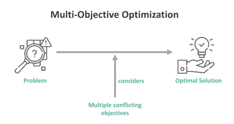
Multi-objective portfolio optimization is a complex and challenging problem in the field of finance and optimization. It involves selecting a combination of assets or investments that maximize multiple conflicting objectives simultaneously. These objectives often include maximizing returns, minimizing risk, and achieving other financial goals. The main idea is to find a balance between different objectives, as improving one objective may lead to a trade-off with another.

In traditional single-objective portfolio optimization, the goal is to either maximize returns for a given level of risk or minimize risk for a given level of returns. In multi-objective optimization, there can be more than two objectives related to returns, risk, liquidity, and other financial metrics. Constraints may include limitations on asset allocation, sector exposure, or any other regulatory or investor-specific requirements.

History (cause, why not)

Multi-Objective Portfolio Optimization can be pictured as a financial adventure through time. It started around the 1950s with a financial wizard named Harry Markowitz. He had this wild thought to find the perfect mix of investments that would give you the most money while keeping minimal risk of losing it.

Then in the ’80s and ’90s, along came computers that made things way easier. People started using computer programs to figure out how to invest their money most smartly. It’s as if you have a super-smart assistant figuring everything out for you.

Moreover these days it isn’t only about making money but there are other things like caring about the planet (called ESG investing) or paying less tax. So, now, it’s like trying to bake that same cake, but you also want it to be healthy (like being eco-friendly) and not too expensive (like saving taxes).

Moving on to the present, it’s not just computers helping us but there are super-smart machines that can process billions of pieces of information to help you make the best investment choices ( called machine learning ). It’s like having a superhero sidekick in the world of finance, making sure your money works hard for you.

Subject to market risks, read all scheme-related documents carefully xD

Mathematical Optimisation (Fair warning: very boring)

The mathematical formulation of multi-objective portfolio optimization involves defining objective functions, decision variables, and constraints. Below is a simplified representation of the mathematical model for multi-objective portfolio optimization:

Objective Functions:

For the mathematical part, consider k different objective functions f1(x), f2(x), …,fk(x) where x is the vector of decision variables representing the portfolio weights.

Typically, the objectives include maximizing returns and minimizing risk, but they can also include other financial or non-financial goals. These objectives are:

f1(x): the return objective, e.g., maximizing expected portfolio return.
f2(x): the risk objective, e.g., minimizing portfolio risk (variance or standard deviation).
f3(x): represents additional objectives such as achieving a target level of risk-adjusted return, sector exposure constraints, or other specific criteria.

Decision Variables:

Let x be a vector of decision variables representing the portfolio weights assigned to each asset in the portfolio. The sum of these weights should equal 1 to ensure that the portfolio is fully invested.

sum(x1,x2, ….., xn) = 1

Where xi is the weight of i-th asset in the portfolio and n is the total number of assets.

Constraints:

The sum of all weights should always be equal to 1.
Minimum and maximum investment limits for all assets their weights should be xmin ≤ x ≤ xmax
Other constraints like constraints on sector exposure, asset class exposure, or other specific requirements.

Solving the problem:

To solve the multi-objective problem, you need to find a set of portfolio weights (x) that optimizes the multiple objective functions simultaneously. This often involves trade-offs between the objectives, and different mathematical techniques can be used to address this trade-off, such as scalarization methods.

A common approach is to use scalarization to convert the multi-objective problem into a single-objective problem by using weighted combinations of the objectives. For example, you can create a weighted sum of the objectives:

Z = w1⋅f1(x) + w2⋅f2(x) +……. + wk⋅fk(x)

We then maximize the function Z by adjusting the weights w1, w2, .., wk

Here, w1, w2, .., wk are weights representing the importance of each objective.

Adjusting these weights allows you to explore the trade-offs between objectives and find different solutions on the Pareto front.

*The Pareto front represents a set of solutions where one objective cannot be improved without degrading another. It illustrates trade-offs between conflicting objectives.

Example

For ease of understanding, let’s take two objectives instead of more.

Next, we continue with the following steps:

Step 1: Define the Objective Function:

The objective function is a mathematical expression that quantifies what you want to maximize or minimize. It typically involves decision variables.

For our assets:

W1: Weight of asset 1
W2: Weight of asset 2
m1: Expected returns of asset 1
m2: Expected returns of asset 2
s1: Standard Deviation of asset 1
s2: Standard Deviation of asset 2
c: Correlation between asset 1 & asset 2

Our Objective Functions:

Maximize: f1(w) = m1*w1+m2*w2 (Maximize expected return)

Minimize: f2(w) = w12 *s12 + w22 *s22 + 2*c*w1*w2*s1*s2 (Minimize portfolio variance. c is the correlation coefficient between Asset 1 and Asset 2)

Step 2: Identify Decision Variables:

Decision variables are the parameters you want to optimize. They are often denoted by symbols (e.g., x, y, w) and can represent quantities, allocations, or actions.

Step 3: Specify Constraints:

Constraints are conditions or limitations that must be satisfied. They can be equations or inequalities involving the decision variables.

Here the constraints are:

w1 + w2 = 1: The sum of weights is equal to 1.
w1,w2 >=0: Non-negativity constraint for each weight

Step 4: Formulate the Optimization Problem:

Combine the objective function and constraints to create a comprehensive mathematical expression.

Our overall question:

Maximize: Z = a*f1(w) — (1-a)*f2(w) {where a is the weighting parameter}

Subject to:

w1 + w2 = 1
w1,w2 >=0

Step 5: Choose the Optimization Technique:

Select the appropriate optimization method for solving the problem. Common techniques include linear programming (LP), quadratic programming (QP), mixed-integer linear programming (MILP), nonlinear programming (NLP), and more.

Step 6. Solve the Optimization Problem:

Apply the chosen optimization technique to find the optimal solution. Software packages like MATLAB, Python (using libraries like SciPy), or specialized optimization solvers can be used.

Step 7: Evaluate the Solution:

After solving the optimization problem, you will obtain values for the decision variables. Evaluate the objective function to determine the optimal value.

In our example, we assumed:

m1 = 0.08, m2 = 0.12
s1 = 0.15, s2 = 0.27
c = 0.3

Optimal Solution (wi*):

w1* = 0.321, w2* = 0.679

Optimal Value: Z* = 0.065

Run the full mathematical model whose code is attached here: Model

Step 8: Interpret the Results:

Understand the implications of the optimal solution in the context of your problem. Does it make sense given your objectives and constraints?

The above steps provide a simplified overview of the process. In practice, optimization problems can be much more complex, involving nonlinear objective functions, multiple constraints, and discrete variables. The specific formulae and methods used will depend on the nature of the problem and the chosen optimization technique.

If you reached till here and are reading this sentence, I sincerely appreciate your patience. Let us reward you by showing how you can apply this to your portfolio.

Implementation (since theory will take you only so far)

We looked into the history and definition. Now let's learn the implementation of Multi-Objective Portfolio Optimisation.

Step 1: Define your Objectives and their Constraints

- Start by listing your investment objectives. For example, we want to maximize returns and minimize risk here, but you can customize the objective as per your requirements.

- Specify needed constraints such as the total investment amount, asset allocation limits, and target minimum return.

Step 2: Collection of Data

- Gather historical data on the assets you want to include in your portfolio. This data should include all the past returns and risks (standard deviations) for each asset.

Step 3: Calculate Expected Returns and Risks

- Calculate the expected return and risk for each asset based on the historical data. The expected return is typically the average historical return, and risk is the standard deviation of returns.

Step 4: Create a Portfolio

- Create a table with different random portfolio combinations of assets. Vary the allocation percentages(weight) for each asset to cover a wide range of possibilities.

- Calculate the portfolio return and risk for each combination using weighted averages.

Step 5: Efficient Frontier

- Create a scatter plot with portfolio risk (x-axis) and return (y-axis).

- Plot each portfolio combination as a point on the graph.

- Use the best fitting line or curve to connect the points that represent the best trade-offs between risk and return. This curve is known as the Efficient Frontier*.

* The efficient frontier is a concept in finance that represents the set of optimal portfolios offering the highest expected return for a given level of risk, or the lowest risk for a given level of expected return. It illustrates the trade-off between risk and reward in portfolio optimization.

Step 6: Optimization

- Implement mathematical optimization algorithms (e.g., quadratic, linear programming) to find the portfolios on the Efficient Frontier that best aligns with your objectives and constraints.

- These portfolios are known as Pareto-optimal portfolios.

Step 7: Plot Pareto-optimal Portfolios

- On the Efficient Frontier graph, plot the Pareto-optimal portfolios obtained through optimization. These are the portfolios that represent the best return-to-risk ratio.

Step 8: Choose a Portfolio

- Depending on your risk tolerance and return requirements, select one of the Pareto-optimal portfolios from the graph.

- This chosen portfolio will be the optimal allocation of assets that aligns with your required objectives and constraints.

Code Implementation of MOPO:

Overview of Code

Before jumping to the full code implementation let us look at an overview of what we are trying to do with the code and then we will move on to the actual code.

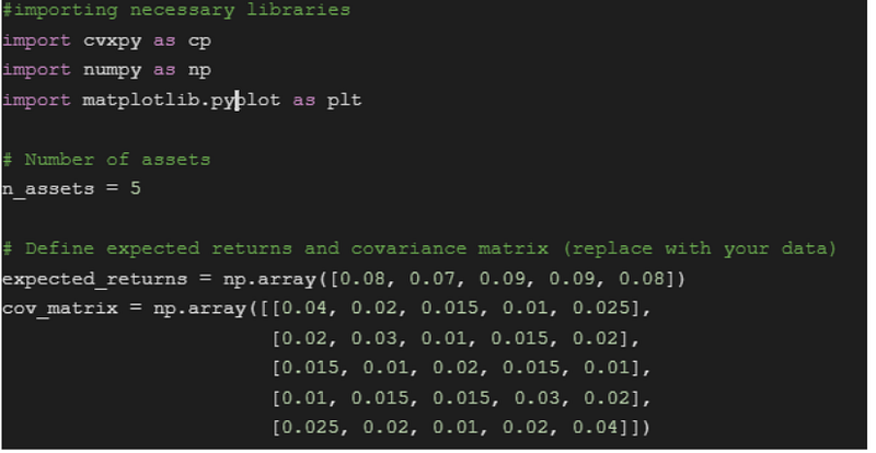
We start by importing the necessary libraries such as numpy, matplotlib and cvxpy. Cvxpy is used to formulate and solve convex optimization problems.

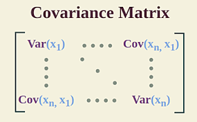
2. Then we decide on how many assets(‘n_assets’) we want to consider and then save their expected returns (‘expected_returns’) in an array. We saved the covariance among the assets in a matrix (‘cov_matrix’)

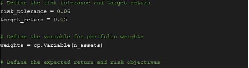
3. We then defined the maximum allowed portfolio risk (variance) which is ‘risk_tolerance’ and the desired level of expected return from the portfolio ‘target_return’.

4. The weights of the assets in the portfolio are represented by ‘weights’ and it is declared as a cvxpy.Variable.

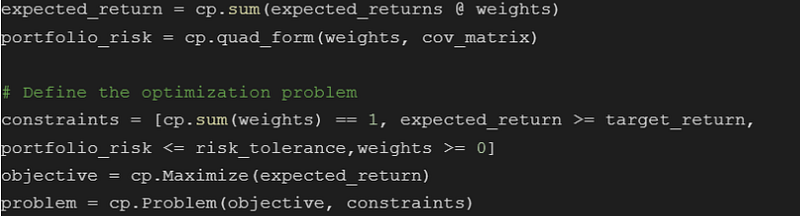
5. Then we define ‘expected_return’ which is calculated as the sum of expected returns weighted by the portfolio weights and ‘portfolio_risk’ is defined using the quadratic form to calculate portfolio risk (variance).

6. Then we set the constraints for the model to train. The constraints are:

The sum of all weights should be 1 (fully invested portfolio)
All the weights should be greater than equal to 0 (only long positions)
The expected return should be more than or equal to the target return
Portfolio risk should be less than equal to risk tolerance.

7. Defined the objective which is to maximize the expected return.

8. Create this problem using the ‘cvxpy.Problem’ and the arguments as ‘objective’ and ‘constraints’.

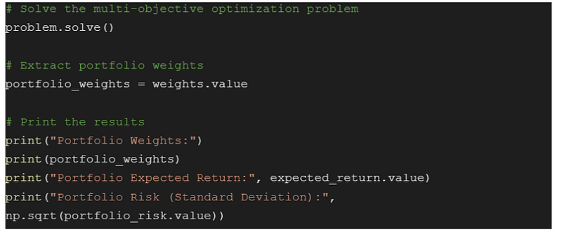
9. Solve the multi-objective optimization problem using ‘problem.solve()’. This finds the portfolio weights that maximize expected return while satisfying constraints. Extract and print the portfolio weights, expected return, and risk (standard deviation) of the portfolio.

10. Extract and print the portfolio weights, expected return, and risk (standard deviation) of the portfolio.

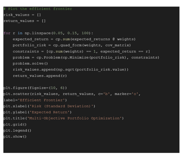
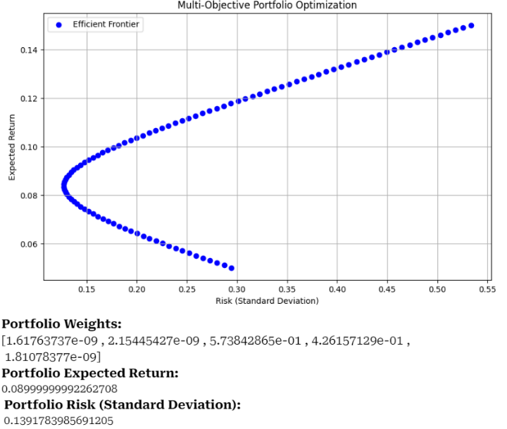
11. Calculate and plot the efficient frontier.

Now, THE CODE (literally)

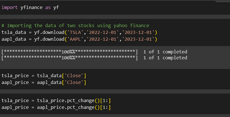
Firstly, to form the covariance matrix, we took stocks of Apple and Tesla and imported their closing price data from Yahoo Finance.
We then took the percentage difference in prices between adjacent row cells using pct_change.

To calculate the expected return, we applied the below formula (.shift(1) shifts down the data by one row downward since the change in returns is calculated by ret(t+1)-ret(t)/ret(t))

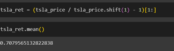
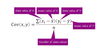
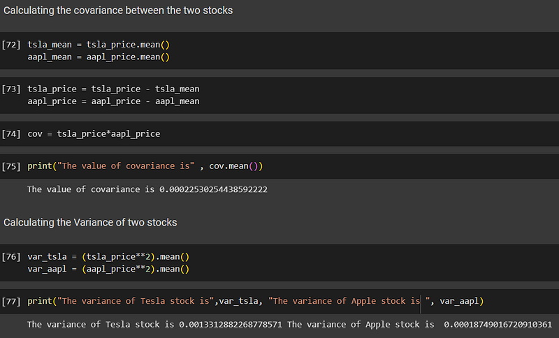
We then calculated the mean and used the covariance formula mentioned above to calculate variance as well as covariance for both stocks. Similarly, we can calculate the covariance between multiple other stocks.

Importing necessary libraries, defining total assets and taking our expected returns as well as covariance matrix(here we took 5 other stocks for our portfolio and calculated their covariance matrix as well as expected returns)

Defining returns, risk, variable weights, as well as the optimisation problem(setting the total sum of weights=1)

Solving the problems and printing the optimized weight distribution

Plotting the efficient frontier(max risk and return combination)

Other outcomes (flexing our visualisation skills tbh)

By plotting the return vs risk graph using randomly generated weights we find the whole feasible region with the leftmost boundary as our efficient frontier.
Taking more and more points in each step, here’s a simulation of returns vs risk plot with randomly generated weights for better visualization of the efficient frontier.

Simulation shows Expected Return vs Risk for randomly generated weights, the leftmost boundary being the efficient frontier.

Run the full code here: CODE-MOPO

Conclusion and Insights

Unlike single objective portfolio optimisation, there is no single best solution of MOPO, but a range of solutions with different risks and returns.
It doesn’t directly optimize risk and return but takes in a variety of utility functions to cater to the preferences of the investor.
It can consider goals not only associated with financial metrics, but also specific wealth, retirement readiness, or philanthropic targets.
Investors can try and test different economic markets to see how the portfolios perform.
Investors can explore efficient frontier for multiple objectives simultaneously, often having conflicting goals.
It also has a dynamic setting which helps it to keep itself updated with the trends.
MOPO considers trading costs as well as liquidity constraints which single objective portfolio optimisation doesn’t.

While MOPO in itself, is a commendable and powerful tool, it also has some downsides.

Complexity- Due to its multi-objective ability, this requires specialized tools and algorithms to implement.
Ambiguity — MOPO results in a range of solutions with various parieto-optimal solutions, selecting the best solution can be difficult.
Data accuracy- The input data (returns, volatility, correlations) are very sensitive and significantly impact the optimization results.
Runtime — Solving MOPO problems can be computationally intensive, especially for large portfolios and complex objectives.

All in all, Multi-Objective Portfolio Optimisation redefines investment decisions by harmonizing risk, return and diverse objectives. Through Pareto-Efficient Solutions it helps the portfolio to have a balanced trade-off, thus helping him/her to make personalized, optimum and informed strategies.

This brings us to the end of this simple yet elegant concept. Hope you guys found this read insightful. We’ll be back with more so stay tuned!

References

FIN.