Portfolio Optimisation using Monte Carlo Simulation

Overview

In today’s volatile financial markets, optimizing an investment portfolio is essential to achieve the desired balance between risk and return. Monte Carlo simulations offer a powerful tool to assess different asset allocation strategies and their potential outcomes under uncertain market conditions.

Objective

The objective of this project is to develop a Monte Carlo simulation model for portfolio optimization. Participants will be required to construct and analyze portfolios composed of various asset classes (e.g., stocks, bonds, and alternative investments) to maximize expected returns while managing risk.

Model

Data Collection & Pre-Processing: Collected data from Kaggle about the asset’s prices, and used the CSV files for analysis. One may also use yfinance to get access to real-time stock prices within a fixed time frame (b/w start & end date).

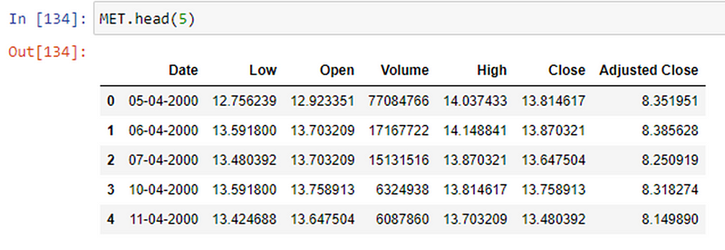
Then coming onto pre-processing I focused on analyzing the ‘Adjusted -Close’ of the stocks due to a number of factors. The “Adjusted Close” section of the data, means the cash value of the last transacted price before the market closes. The adjusted closing price is attributed to anything that would affect the stock price after the market closes for the day.

The adjusted closing price of the stock helps investors know the fair value of the stock after the corporate action is announced and also helps maintain an accurate record of where the stock price starts and where it ends so we choose to the analysis of it instead of the closing price.

Visualization

To get more insights into the stocks being used how they relate to one another, and how change in one affects the other. This would help an investor diversify the portfolio thus minimising the risk. Diversification is important as it helps the investor when the market goes down, thereby some stocks may nullify the losses incurred by the rest of the assets.

For this, I plotted a heatmap of Covariance and Correlation

Correlation, in the finance and investment industries, is a statistic that measures the degree to which two securities move in relation to each other.

You can think of correlation as a scaled version of covariance, where the values are restricted to lie between -1 and +1. A correlation of +1 means positive relation, i.e, if the correlation between Asset A and Asset B is 1, if Asset A increases, Asset B increases. And 0 means no relation.

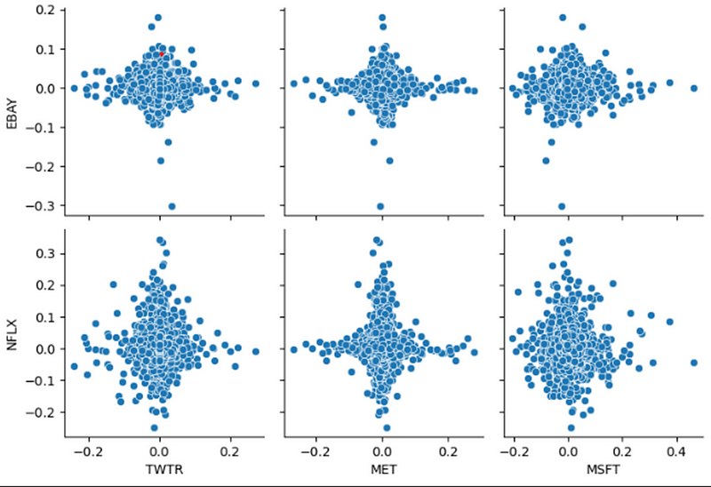
Seaborn’s pairplot() function is used to create a scatter plot matrix. In this matrix, you can see how variables within the stock_returns are related pairwise. The resulting plot can provide insight into the correlations and patterns between the daily returns of different companies.

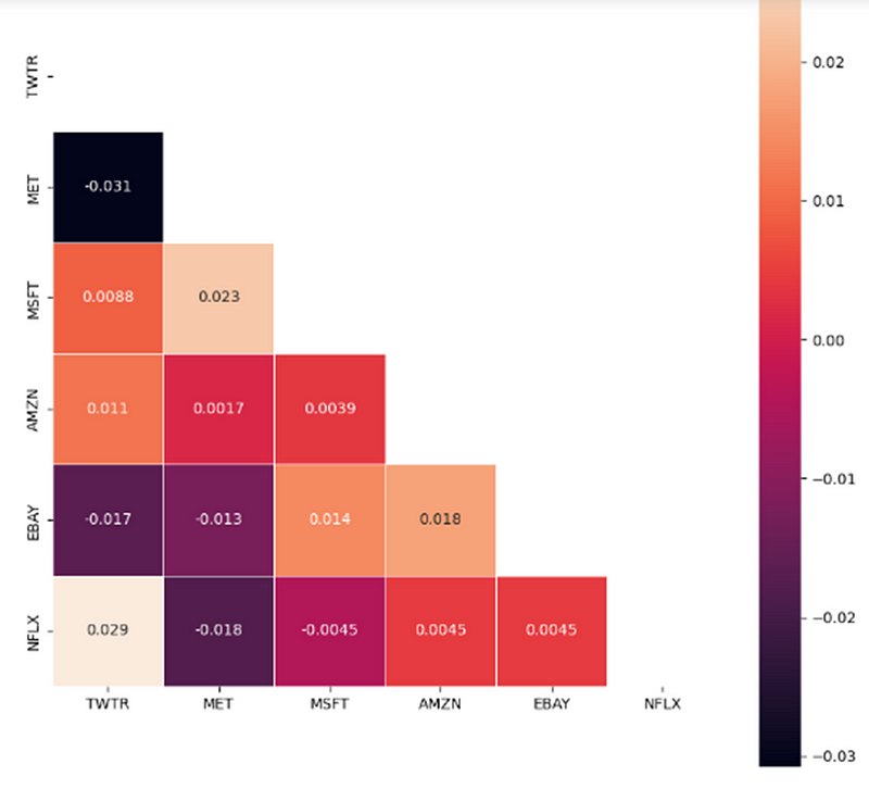
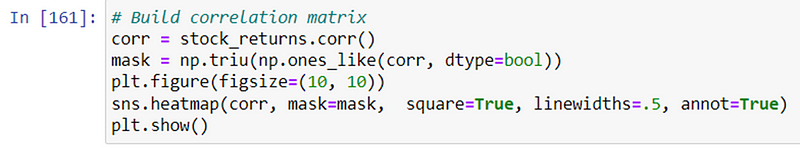
A heatmap plot is generated to visualize the correlations between stock_returns and the correlation matrix created in the provided code snippet.

Log Returns vs Simple Returns

We usually prefer log returns over simple returns due to the following reasons.

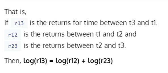
1. Its time additive.
2. It follows a normal gaussian distribution

We can also see from the histogram of log returns, it’s mostly centered around 0, looks a bit normally distributed.

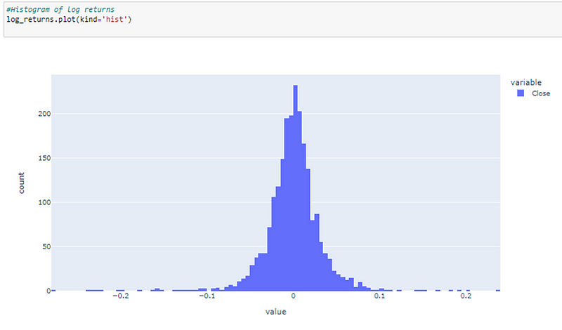
But there is quite a catch here is normality a good assumption for financial data? The assumption that prices or more accurately log returns are normally distributed.

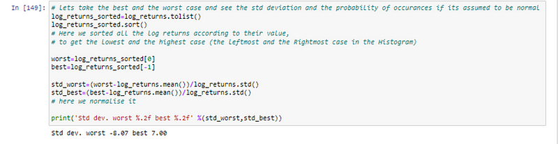
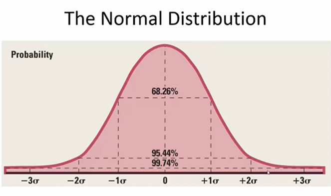
As we can see the deviation is huge, as in normal distribution about 99.75% of the data is within 3 standard deviations, which is just not the case here. But how do we actually test for normality and how good to approximate it as gaussian.

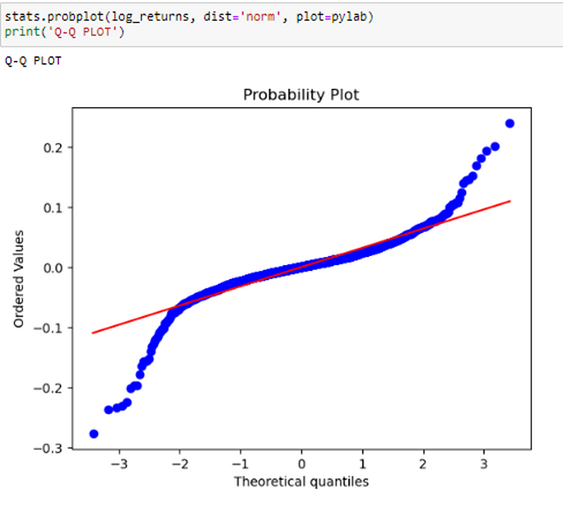
As we can see from here normally treating financial data as normally distributed is not a bad assumption for the most part, except for the tails. Which we can see from the plot as well, at the tails and heads there seems a deviation from normality.

We can also prove log returns are additive by observing that when we add the log returns over the whole course, we get the closing price.

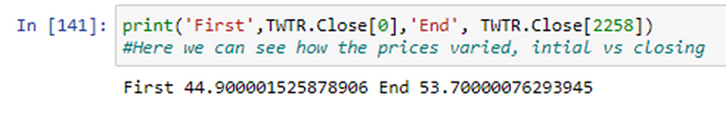
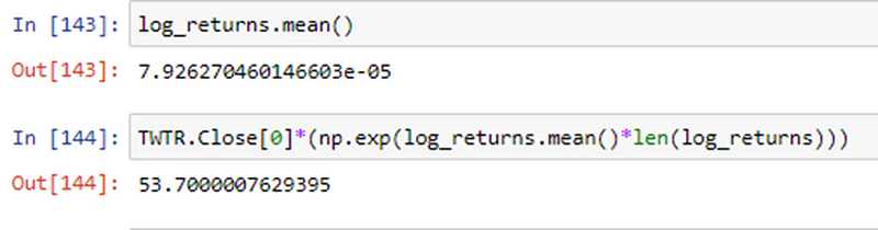
Which we can see from the above snippet that log returns exactly predicts it.

Whereas if we were to use simple returns then,

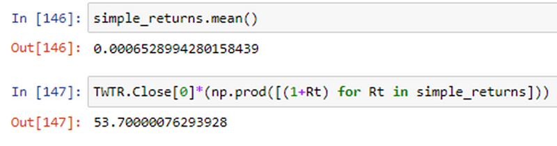
As we can see those simple returns although gave a prediction to the actual value but not the actual value due to the fact that product of normally distributed variables is not normally distributed.

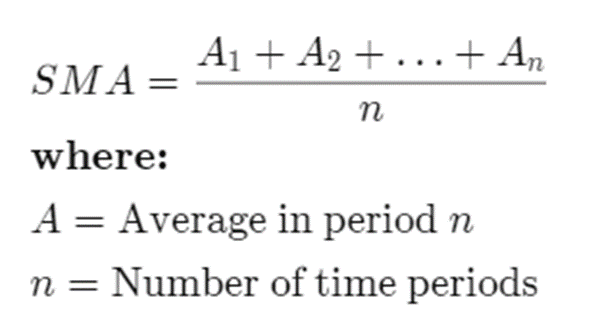
Simple Moving Average(SMA)

Moving averages were incorporated to eliminate fluctuations and reduce the number of variations present in the data. This process is called the smoothening of time series.

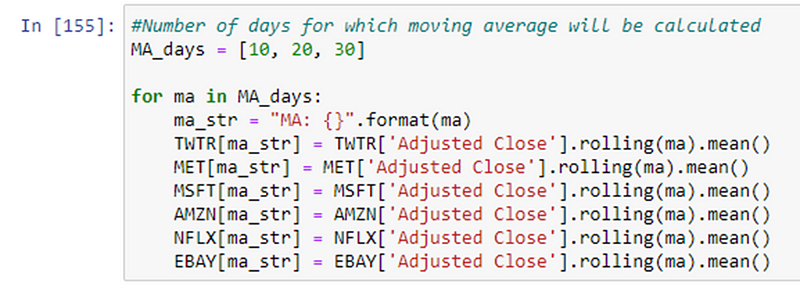
I have used 10,20,30 days moving averages, Shorter moving averages are typically used for short-term trading whereas long ones are for long-term trading.

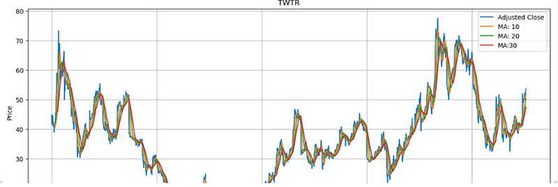
As we can see above, that the line gets more and more smooth as we take a greater number of days into consideration. Thus, when we take a greater number of days into consideration, then the line becomes more laggy to fluctuations.

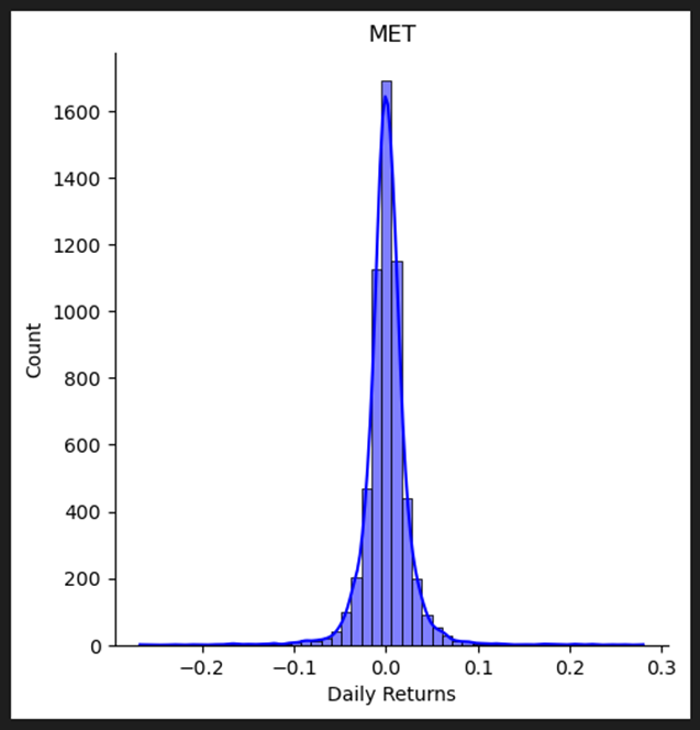
Calculating returns and draw distribution

This code snippet calculates the daily returns for each company within the data list and visualizes the distribution of these returns using a histogram.

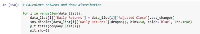
On observing we see it follows almost a normal distribution, we say “almost” as on the head and tail parts of the histogram (upon which we did smoothening to arrive at this conclusion) don’t follow gaussian distribution very strictly (why? And how can we say this? I have explained this in my talk of normality section)

Random shares, combinations, and Max Sharpe Ratio

The provided code defines a function called randomPortfolio() that is responsible for generating a random portfolio of shares.

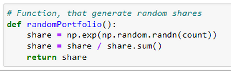
It generates a random portfolio of shares by drawing random values from a standard normal distribution, exponentiating them to ensure positive values, and then normalizing them to represent proportions of the total portfolio value. By calling this function, you can obtain a random allocation of shares for a portfolio.

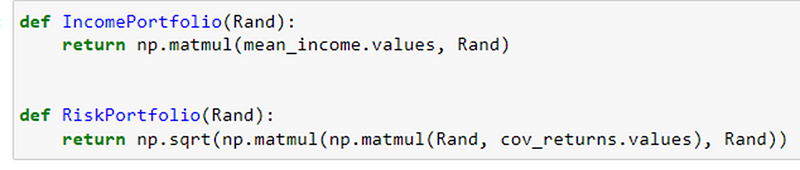
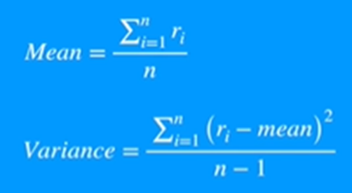
IncomePortfolio(Rand) and RiskPortfolio(Rand). These functions are designed to perform calculations related to income and risk for a portfolio.

The IncomePortfolio(Rand) function calculates the expected income of a portfolio based on the mean income values and the allocation of assets. The RiskPortfolio(Rand) function, on the other hand, calculates the risk of a portfolio based on the covariance matrix of returns and the allocation of assets. Together, these functions provide essential metrics for evaluating the income and risk characteristics of a portfolio.

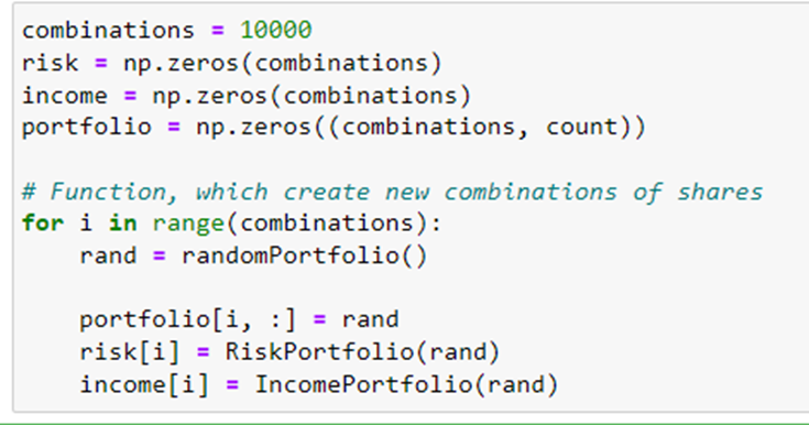
First, the variable “combinations” is initialized to 10000. This variable determines the number of portfolio combinations that will be generated and evaluated

Next, three arrays named “risk,” “income,” and “portfolio” are created and initialized with zeros. These arrays will store the risk, income, and portfolio data for each combination.

The randomly generated portfolio is then assigned to the ith row of the “portfolio” array. Each row in the “portfolio” array represents a different combination of shares.

Next, the “RiskPortfolio()” function is invoked, passing the current portfolio as an argument. This function calculates the risk associated with the given portfolio.

Following that, the “IncomePortfolio()” function is called with the current portfolio as an argument. This function computes the income or expected return of the portfolio.

The ratio is the average return earned in excess of the risk-free rate per unit of volatility or total risk. Volatility is a measure of the price fluctuations of an asset or portfolio.

The risk-free rate of return is the return on an investment with zero risk, meaning it’s the return investors could expect for taking no risk.

The optimal risky portfolio is the one with the highest Sharpe ratio.

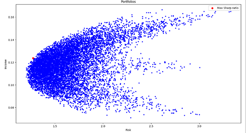
The maximum Sharpe ratio by adding a red dot at its corresponding risk and income values and including a legend to identify it. The scatter plot provides a visual representation of the risk and income relationship for the portfolios.

Best portfolio is one with the Max Sharpe Ratio and its weights can also be fetched.

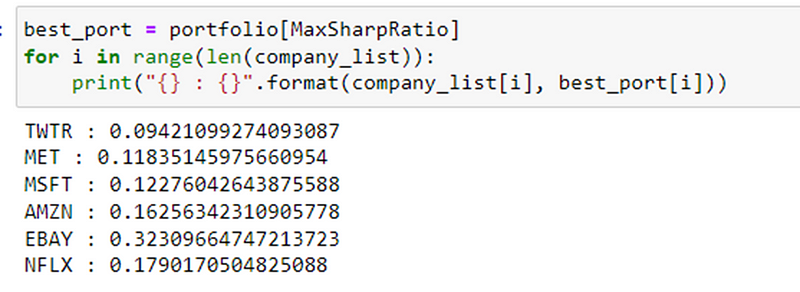
This code identifies the portfolio with the highest Sharpe ratio and then displays the allocation or weight assigned to each company in that portfolio. It allows us to see how the assets or companies are distributed within the best-performing portfolio.

Future price predictions using Monte Carlo Simuation

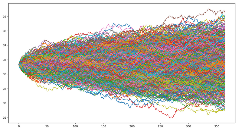
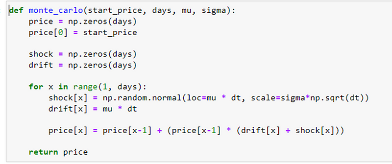
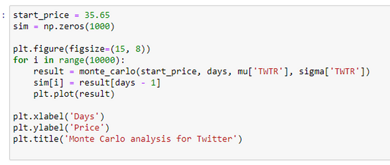
The provided code snippet introduces a function named monte_carlo that employs the Monte Carlo method to simulate the future price of a stock.

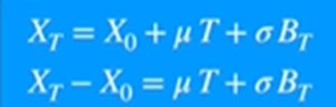
For the generation of random paths, I have used arithmetic Brownian motion, instead of this one can use geometric Brownian motion too.

The more the variance the more the spread is, and the less the steepness is.

In context to Monte Carlo Simulation, the random paths generated would be less differentiating if the variance is less and it would be more if the variance is more resulting in a flatter curve.

The monte_carlo function uses the Monte Carlo method to generate simulated stock prices for a specified number of days. It considers the initial stock price, average daily return, and standard deviation of daily returns. The function incorporates random shocks and drift components to calculate the simulated prices for each day.

This code performs a Monte Carlo analysis of Twitter’s stock by predicting its future prices through 1000 simulations. The final prices from these simulations are stored in the ‘sim’ array and plotted. By doing so, the code offers potential insights into the future price range of Twitter’s stock, as determined by the Monte Carlo simulations.

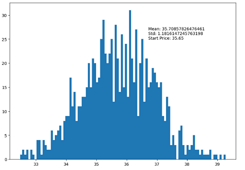
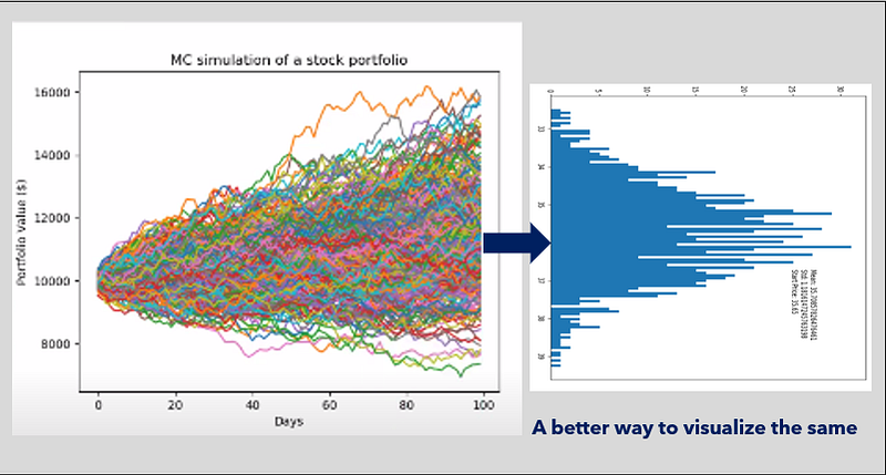
The provided code constructs a histogram to illustrate the distribution of the Twitter stock’s simulated prices derived from the Monte Carlo simulations. The visualization includes text annotations that outline the mean, standard deviation, and initial price of the simulated prices. This visual representation provides valuable insights into the potential range and traits of Twitter’s future stock prices, as per the Monte Carlo simulations.

Further recommendations:

1. Incorporate measures of normalities like Q-Q plot (used above), Box Plots, Kolmogonov Smirmov Test to quantify normality, this would help in visualizing the quantification of the normality of the data.
2. Usage of the Exponential moving average(EMA) the calculation for EMA emphasizes the recent data points. EMA responds more quickly to changing prices than the Simple Moving Average(SMA).
3. Effect of number of days taken into account during the calculation of moving average and how it affects the smoothening.
4. Use other Risk-Return measures such as the Sortino Ratio, M2 Ratio, Calmar Ratio and calibrate their differences, and use the most suitable one according to the scenario.
5. Usage of Geometric Brownian Motion(GBM) instead of Arithmetic Brownian Motion(ABM) for the generation of randomized paths which would be fed into the Monte Carlo Simulation.
6. Observe how changing the risk factor affects the optimal portfolio.

For the codebase, you may refer to my Github https://github.com/beingamanforever/Monte-Carlo-Simulation

References used:

1. Investopedia
2. QuantPie yt channel
3. MIT lectures on Monte Carlo simulation