Free AI web copilot to create summaries, insights and extended knowledge, download it at here
8609
Abstract
6401</span>
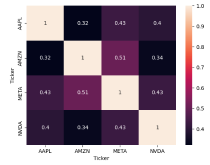
NVDA <span class="hljs-number">0.398202</span> <span class="hljs-number">0.335418</span> <span class="hljs-number">0.426401</span> <span class="hljs-number">1.000000</span>
<span class="hljs-keyword">import</span> seaborn <span class="hljs-keyword">as</span> sns
ax = sns.heatmap(corr_matrix, annot=<span class="hljs-literal">True</span>)</pre></div><figure id="9c90"><img src="https://cdn-images-1.readmedium.com/v2/resize:fit:800/1*nmOAgrT7SMwDBQZ6HtCo5Q.png"><figcaption>Correlation matrix of log daily changes</figcaption></figure><ul><li>Calculating the randomly weighted portfolio’s variance</li></ul><div id="b41c"><pre>w = {<span class="hljs-string">'AAPL'</span>: <span class="hljs-number">0.1</span>, <span class="hljs-string">'NVDA'</span>: <span class="hljs-number">0.4</span>, <span class="hljs-string">'META'</span>: <span class="hljs-number">0.3</span>, <span class="hljs-string">'AMZN'</span>: <span class="hljs-number">0.2</span>}
port_var = cov_matrix.mul(w, axis=<span class="hljs-number">0</span>).mul(w, axis=<span class="hljs-number">1</span>).<span class="hljs-built_in">sum</span>().<span class="hljs-built_in">sum</span>()
port_var
<span class="hljs-number">0.0005679211473087001</span></pre></div><ul><li>Calculating the yearly returns for individual stocks</li></ul><div id="d41b"><pre>ind_er = df.resample(<span class="hljs-string">'Y'</span>).last().pct_change().mean()
ind_er
Ticker
AAPL <span class="hljs-number">0.333813</span>
AMZN <span class="hljs-number">0.688729</span>
META <span class="hljs-number">0.414315</span>
NVDA <span class="hljs-number">0.632646</span>
dtype: float64</pre></div><ul><li>Calculating the portfolio return</li></ul><div id="e79e"><pre>w = [<span class="hljs-number">0.1</span>, <span class="hljs-number">0.4</span>, <span class="hljs-number">0.3</span>, <span class="hljs-number">0.2</span>]
port_er = (wind_er).<span class="hljs-built_in">sum</span>()
port_er
<span class="hljs-number">0.5596969011447753</span></pre></div><ul><li>Calculating the annual std</li></ul><div id="f1e7"><pre>ann_sd = df.pct_change().apply(<span class="hljs-keyword">lambda</span> x: np.log(<span class="hljs-number">1</span>+x)).std().apply(<span class="hljs-keyword">lambda</span> x: xnp.sqrt(<span class="hljs-number">250</span>))
ann_sd
Ticker
AAPL <span class="hljs-number">0.448354</span>
AMZN <span class="hljs-number">0.554643</span>
META <span class="hljs-number">0.402217</span>
NVDA <span class="hljs-number">0.596450</span>
dtype: float64</pre></div><ul><li>Creating a table for visualizing returns and volatility of assets</li></ul><div id="c706"><pre>assets = pd.concat([ind_er, ann_sd], axis=<span class="hljs-number">1</span>)
assets.columns = [<span class="hljs-string">'Returns'</span>, <span class="hljs-string">'Volatility'</span>]
assets
Returns Volatility
Ticker
AAPL <span class="hljs-number">0.333813</span> <span class="hljs-number">0.448354</span>
AMZN <span class="hljs-number">0.688729</span> <span class="hljs-number">0.554643</span>
META <span class="hljs-number">0.414315</span> <span class="hljs-number">0.402217</span>
NVDA <span class="hljs-number">0.632646</span> <span class="hljs-number">0.596450</span></pre></div><ul><li>Plotting the MPT efficient frontier with 10k random portfolios</li></ul><div id="74be"><pre>p_ret = [] <span class="hljs-comment"># Define an empty array for portfolio returns</span>
p_vol = [] <span class="hljs-comment"># Define an empty array for portfolio volatility</span>
p_weights = [] <span class="hljs-comment"># Define an empty array for asset weights</span>
num_assets = <span class="hljs-built_in">len</span>(df.columns)
num_portfolios = <span class="hljs-number">10000</span>
<span class="hljs-keyword">for</span> portfolio <span class="hljs-keyword">in</span> <span class="hljs-built_in">range</span>(num_portfolios):
weights = np.random.random(num_assets)
weights = weights/np.<span class="hljs-built_in">sum</span>(weights)
p_weights.append(weights)
returns = np.dot(weights, ind_er) <span class="hljs-comment"># Returns are the product of individual expected returns of asset and its </span>
<span class="hljs-comment"># weights </span>
p_ret.append(returns)
var = cov_matrix.mul(weights, axis=<span class="hljs-number">0</span>).mul(weights, axis=<span class="hljs-number">1</span>).<span class="hljs-built_in">sum</span>().<span class="hljs-built_in">sum</span>()<span class="hljs-comment"># Portfolio Variance</span>
sd = np.sqrt(var) <span class="hljs-comment"># Daily standard deviation</span>
ann_sd = sd*np.sqrt(<span class="hljs-number">250</span>) <span class="hljs-comment"># Annual standard deviation = volatility</span>
p_vol.append(ann_sd)
data = {<span class="hljs-string">'Returns'</span>:p_ret, <span class="hljs-string">'Volatility'</span>:p_vol}
<span class="hljs-keyword">for</span> counter, symbol <span class="hljs-keyword">in</span> <span class="hljs-built_in">enumerate</span>(df.columns.tolist()):
<span class="hljs-comment">#print(counter, symbol)</span>
data[symbol+<span class="hljs-string">' weight'</span>] = [w[counter] <span class="hljs-keyword">for</span> w <span class="hljs-keyword">in</span> p_weights]
portfolios = pd.DataFrame(data)
portfolios.head() <span class="hljs-comment"># Dataframe of the 10000 portfolios created</span>
Returns Volatility AAPL weight AMZN weight META weight NVDA weight
<span class="hljs-number">0</span> <span class="hljs-number">0.496109</span> <span class="hljs-number">0.356620</span> <span class="hljs-number">0.377360</span> <span class="hljs-number">0.383954</span> <span class="hljs-number">0.207498</span> <span class="hljs-number">0.031189</span>
<span class="hljs-number">1</span> <span class="hljs-number">0.484475</span> <span class="hljs-number">0.335763</span> <span class="hljs-number">0.326887</span> <span class="hljs-number">0.267905</span> <span class="hljs-number">0.300058</span> <span class="hljs-number">0.105150</span>
<span class="hljs-number">2</span> <span class="hljs-number">0.517491</span> <span class="hljs-number">0.352926</span> <span class="hljs-number">0.279398</span> <span class="hljs-number">0.261404</span> <span class="hljs-number">0.212166</span> <span class="hljs-number">0.247032</span>
<span class="hljs-number">3</span> <span class="hljs-number">0.481427</span> <span class="hljs-number">0.352069</span> <span class="hljs-number">0.220658</span> <span class="hljs-number">0.054611</span> <span class="hljs-number">0.404624</span> <span class="hljs-number">0.320107</span>
<span class="hljs-number">4</span> <span class="hljs-number">0.508543</span> <span class="hljs-number">0.349808</span> <span class="hljs-number">0.323731</span> <span class="hljs-number">0.324500</span> <span class="hljs-number">0.208675</span> <span class="hljs-number">0.143094</span>
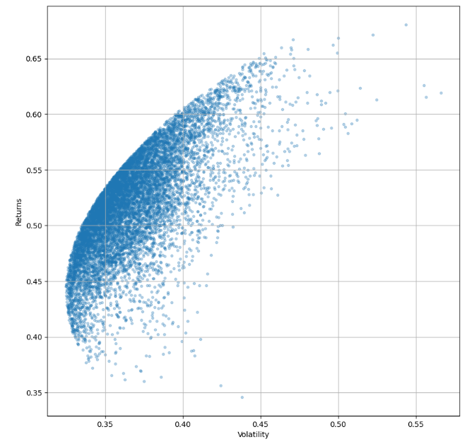
<span class="hljs-comment"># Plot efficient frontier</span>
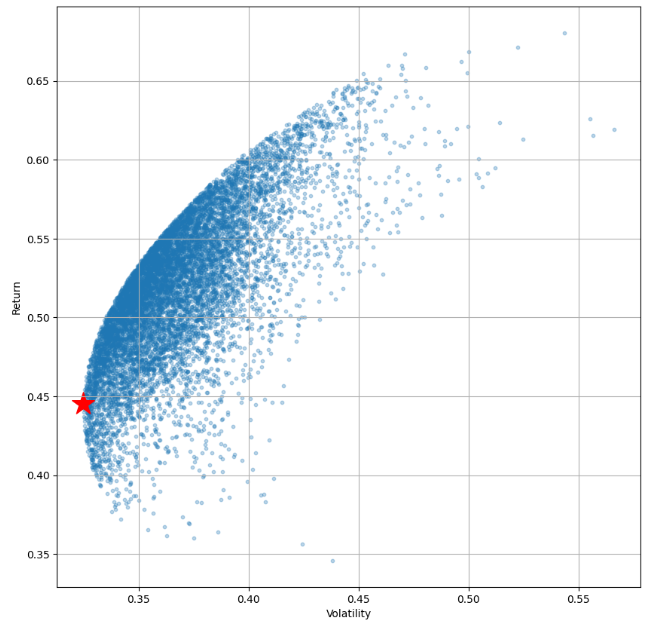
portfolios.plot.scatter(x=<span class="hljs-string">'Volatility'</span>, y=<span class="hljs-string">'Returns'</span>, marker=<span class="hljs-string">'o'</span>, s=<span class="hljs-number">10</span>, alpha=<span class="hljs-number">0.3</span>, grid=<span class="hljs-literal">True</span>, figsize=[<span class="hljs-number">10</span>,<span class="hljs-number">10</span>])</pre></div><figure id="427a"><img src="https://cdn-images-1.readmedium.com/v2/resize:fit:800/1*5K3M_r83UXb3luSnhUtqKw.png"><figcaption>MPT efficient frontier with 10k random portfolios</figcaption></figure><ul><li>The Min Volatility portfolio is as follows:</li></ul><div id="f048"><pre>min_vol_port = portfolios.iloc[portfolios[<span class="hljs-string">'Volatility'</span>].idxmin()]
<span class="hljs-comment"># idxmin() gives us the minimum value in the column specified. </span>
min_vol_port
Returns <span class="hljs-number">0.445058</span>
Volatility <span class="hljs-number">0.324898</span>
AAPL weight <span class="hljs-number">0.327430</span>
AMZN weight <span class="hljs-number">0.145461</span>
META weight <span class="hljs-number">0.448399</span>
NVDA weight <span class="hljs-number">0.078710</span>
Name: <span class="hljs-number">7891</span>, dtype: float64</pre></div><ul><li>Plotting the Min Volatility portfolio</li></ul><div id="73aa"><pre>plt.subplots(figsize=[<span class="hljs-number">10</span>,<span class="hljs-number">10</span>])
plt.scatter(portfolios[<span class="hljs-string">'Volatility'</span>], portfolios[<span class="hljs-string">'Returns'</span>],marker=<span class="
Options
hljs-string">'o'</span>, s=<span class="hljs-number">10</span>, alpha=<span class="hljs-number">0.3</span>)
plt.scatter(min_vol_port[<span class="hljs-number">1</span>], min_vol_port[<span class="hljs-number">0</span>], color=<span class="hljs-string">'r'</span>, marker=<span class="hljs-string">'*'</span>, s=<span class="hljs-number">500</span>)
plt.grid()
plt.xlabel(<span class="hljs-string">'Volatility'</span>)
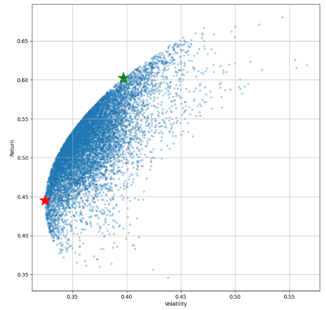
plt.ylabel(<span class="hljs-string">'Return'</span>)</pre></div><figure id="00cb"><img src="https://cdn-images-1.readmedium.com/v2/resize:fit:800/1*ZsLfySmELa345sN1sNkgVQ.png"><figcaption>Min Volatility portfolio vs MPT efficient frontier</figcaption></figure><ul><li>Plotting the max Sharpe ratio portfolio with risk factor of 0.02</li></ul><div id="02db"><pre><span class="hljs-comment"># Finding the optimal portfolio</span>
rf = <span class="hljs-number">0.02</span> <span class="hljs-comment"># risk factor</span>
optimal_risky_port = portfolios.iloc[((portfolios[<span class="hljs-string">'Returns'</span>]-rf)/portfolios[<span class="hljs-string">'Volatility'</span>]).idxmax()]
optimal_risky_port
Returns <span class="hljs-number">0.569114</span>
Volatility <span class="hljs-number">0.371583</span>
AAPL weight <span class="hljs-number">0.050555</span>
AMZN weight <span class="hljs-number">0.386680</span>
META weight <span class="hljs-number">0.321123</span>
NVDA weight <span class="hljs-number">0.241643</span>
Name: <span class="hljs-number">4683</span>, dtype: float64
<span class="hljs-comment"># Plotting optimal portfolio</span>
plt.subplots(figsize=(<span class="hljs-number">10</span>, <span class="hljs-number">10</span>))
plt.scatter(portfolios[<span class="hljs-string">'Volatility'</span>], portfolios[<span class="hljs-string">'Returns'</span>],marker=<span class="hljs-string">'o'</span>, s=<span class="hljs-number">10</span>, alpha=<span class="hljs-number">0.3</span>)
plt.scatter(min_vol_port[<span class="hljs-number">1</span>], min_vol_port[<span class="hljs-number">0</span>], color=<span class="hljs-string">'r'</span>, marker=<span class="hljs-string">''</span>, s=<span class="hljs-number">500</span>)
plt.scatter(optimal_risky_port[<span class="hljs-number">1</span>], optimal_risky_port[<span class="hljs-number">0</span>], color=<span class="hljs-string">'g'</span>, marker=<span class="hljs-string">''</span>, s=<span class="hljs-number">500</span>)
plt.grid()
plt.xlabel(<span class="hljs-string">'Volatility'</span>)
plt.ylabel(<span class="hljs-string">'Return'</span>)</pre></div><figure id="6a6c"><img src="https://cdn-images-1.readmedium.com/v2/resize:fit:800/1*aMW9XNPcwqPx9ysxHv15TA.png"><figcaption>max Sharpe ratio portfolio with risk factor of 0.02, min Volatility portfolio and MPT efficient frontier.</figcaption></figure><ul><li>Plotting the max Sharpe ratio portfolio with risk factor of 0.2</li></ul><div id="1c82"><pre><span class="hljs-comment"># Same as above but with rf = 0.2 </span>
rf = <span class="hljs-number">0.2</span> <span class="hljs-comment"># risk factor</span>
optimal_risky_port = portfolios.iloc[((portfolios[<span class="hljs-string">'Returns'</span>]-rf)/portfolios[<span class="hljs-string">'Volatility'</span>]).idxmax()]
optimal_risky_port
...</pre></div><figure id="0040"><img src="https://cdn-images-1.readmedium.com/v2/resize:fit:800/1*by1XwpMpfi_SMnzAY10UmQ.png"><figcaption>max Sharpe ratio portfolio with risk factor of 0.2, min Volatility portfolio and MPT efficient frontier.</figcaption></figure><ul><li>Notice that while the difference in risk between min Volatility portfolio and max Sharpe portfolio is just ca. 7% (with risk factor of 0.2), the difference in returns is a whopping 15%.</li></ul><h2 id="8967">Conclusions</h2><ul><li>In this post, we have demonstrated how the Markowitz portfolio optimization works in practice.</li><li>We have attempted to balance risk and return of the 4 major tech stocks (tickers): ‘AAPL’, ‘NVDA’, ‘META’, ‘AMZN’.</li><li>The correlation coefficient of these stocks is within the acceptable range [0.32, 0.51].</li><li>The annual std (vol) shows that vol(META)<vol(aapl)<vol(amzn)<vol(nvda).< li=""></vol(aapl)<vol(amzn)<vol(nvda).<></li><li>We have found the following optimal risky portfolio with risk factor of 0.02</li></ul><div id="e5e0"><pre>Returns <span class="hljs-number">0.569114</span>
Volatility <span class="hljs-number">0.371583</span>
AAPL weight <span class="hljs-number">0.050555</span>
AMZN weight <span class="hljs-number">0.386680</span>
META weight <span class="hljs-number">0.321123</span>
NVDA weight <span class="hljs-number">0.241643</span></pre></div><ul><li>Results confirm the key de-risking ability of <a href="https://www.studocu.com/en-us/document/seton-hall-university/corporate-finance/the-advantages-and-limitations-of-markowitz-portfolio-theory/46687042">Markowitz MPT</a> to incorporate the asset correlation matrix into the portfolio optimization process.</li><li>Our future work will focus on <a href="https://www.linkedin.com/pulse/practical-limitations-modern-portfolio-theory-samer-obeidat-mgm">the shortcomings of MPT</a>:</li><li>The model’s underlying assumptions are predicated on <a href="https://www.realized1031.com/blog/what-are-the-advantages-and-limitations-of-the-markowitz-model">normally functioning markets</a>. In highly volatile and unpredictable markets, the model may lose relevance.</li><li>MPT is <a href="https://www.realized1031.com/blog/what-are-the-advantages-and-limitations-of-the-markowitz-model">mean-variance theory</a>. Risk by variance works when returns are normally distributed. Assets that do not follow a normal distribution will not work with the Markowitz Model.</li><li>To mitigate these limitations, we‘ll consider using alternative portfolio optimization methods, such as Black-Litterman <a href="https://fastercapital.com/content/Capital-Scoring-Simulation--How-to-Test-and-Validate-Your-Capital-Scoring-Model-Using-Monte-Carlo-Methods.html">model or Monte Carlo</a> simulation, and incorporate qualitative factors such as market trends and geopolitical <a href="https://fastercapital.com/content/Investment-Risk-Assessment--How-to-Assess-and-Manage-the-Risks-of-Your-Investment-Decisions-and-Strategies.html">risks into our investment decisions</a>.</li></ul><h2 id="f29b">Explore More</h2><ul><li><a href="https://wp.me/pdMwZd-1YB">Stock Portfolio Risk/Return Optimization</a></li><li><a href="https://wp.me/pdMwZd-1Zl">Risk/Return QC via Portfolio Optimization — Current Positions of The Dividend Breeder</a></li><li><a href="https://wp.me/pdMwZd-21T">Portfolio Optimization Risk/Return QC — Positions of Humble Div vs Dividend Glenn</a></li><li><a href="https://wp.me/pdMwZd-26M">Risk/Return POA — Dr. Dividend’s Positions</a></li><li><a href="https://wp.me/pdMwZd-2f2">Bear vs. Bull Portfolio Risk/Return Optimization QC Analysis</a></li><li><a href="https://wp.me/pdMwZd-4Je">Portfolio Optimization of 20 Dividend Growth Stocks</a></li><li><a href="https://wp.me/pdMwZd-4TI">Applying a Risk-Aware Portfolio Rebalancing Strategy to ETF, Energy, Pharma, and Aerospace/Defense Stocks in 2023</a></li><li><a href="https://wp.me/pdMwZd-5E7">Risk-Aware Strategies for DCA Investors</a></li><li><a href="https://wp.me/pdMwZd-4IB">Towards Max(ROI/Risk) Trading</a></li></ul><h2 id="9156">References</h2><ul><li>Markowitz, Harry, 1952, Portfolio selection, Journal of Finance 7, 1, 77–91.</li><li><a href="https://ryanoconnellfinance.com/python-portfolio-optimization/">Portfolio Optimization using Python and Modern Portfolio Theory</a></li><li><a href="https://readmedium.com/portfolio-optimization-a-beginners-guide-24488cebf52c">Portfolio Optimization: A Beginner’s Guide.</a></li><li><a href="https://readmedium.com/portfolio-optimisation-using-monte-carlo-simulation-25d88003782e">Portfolio Optimization using Monte Carlo Simulation</a></li><li><a href="https://github.com/damianboh/portfolio_optimization/blob/main/Max%20Sharpe%20Ratio%20Portfolio%20Optimization%20for%20Stocks%20Using%20PyPortfolioOpt.ipynb">Optimize portfolio for max Sharpe ratio plot it out with efficient frontier curve</a></li></ul><h2 id="f5d8">Contacts</h2><ul><li><a href="https://newdigitals.org/">Website</a></li><li><a href="https://github.com/alva922">GitHub</a></li><li><a href="https://twitter.com/alzapress">X/Twitter</a></li><li><a href="https://nl.pinterest.com/alexzap922/">Pinterest</a></li><li><a href="https://mastodon.social/@alexzap">Mastodon</a></li><li><a href="https://alva922.tumblr.com/">Tumblr</a></li></ul></article></body>