Portfolio Optimization of 4 Major Techs: Markowitz, Sharpe, VaR & CAPM

This article outlines a stochastic approach to investment portfolio optimization using several key KPIs and underlying models for maximizing the ratio RRR, where RRR=Return/Risk.
Specifically, we will walk through the Markowitz Efficient Frontier, Monte Carlo portfolio simulations, and the CAPM Line Alpha & Beta Monthly Returns in Python.
Our goal is to build and compare the max Sharpe ratio, the min VaR, and the min Volatility (Vol) portfolios for 4 major tech growth stocks such as NVDA, META, AMZN, and AAPL.

Business Case / Motivation

Notably, Apple has achieved a remarkable feat by surpassing a $3 trillion market cap, making it the sole company in recorded history to reach this milestone. Read more here.
If you’re considering entering the eCommerce market, it’s important to note that AMZN currently commands 37.8% of the US eCommerce market share, demonstrating its significant dominance in the industry.
Recent revenue growth reports suggest that META is still a major player in the digital advertising market, and that it is well-positioned for future growth.
In 2023, NVDA saw a remarkable surge in its share price by 228%, reaching a market capitalization of a staggering $1.19 trillion. This impressive financial performance is reflective of the company’s strategic shift from a gaming-focused business to designing chips for self-driving and driver-assisting vehicle technologies, cloud computing, and data centers. In fact, the data segment has now become the largest revenue generator for the company. Read full story.

A Lean Environment Setup

Set up a lean, robust data science environment with Miniconda and Conda-Forge
Download and install Miniconda
conda create -n my-conda-env
conda install jupyter
jupyter notebook
For installing multiple packages from the command line, just pass them as a space-delimited list, e.g.:
pip install package1, package2, …
conda deactivate (exit)
Jupyter Notebook: Setting up the working directory YOURPATH

import os
os.chdir('YOURPATH')    # Set working directory
os. getcwd()

Basic Imports

import pandas as pd
import numpy as np
from functools import reduce
import yfinance as yfin
from pandas_datareader import data as pdr
import yfinance as yf 
import datetime
import random
import scipy.optimize as sco
from scipy import stats
import matplotlib.pyplot as plt
import matplotlib as mpl
import seaborn as sns
%matplotlib inline
mpl.style.use('ggplot')
figsize = (15, 8)
yf.pdr_override()

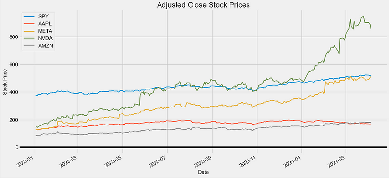
Input Stock Data Analysis

Downloading tech stock data and exporting as CSV

tickers = ("SPY", "AAPL", "META", "NVDA", "AMZN") 

start = "2023-01-03"
end = '2024-04-05'

fin_data = yfin.download(tickers, start, end) #download yahoo finance data for specific dates

fin_data.to_csv('fin_data.csv') #convert data to csv

#check the dimensions of the data
fin_data.shape
(315, 30)
#view the last 5 rows of the data
fin_data.tail()
Price Adj Close Close ... Open Volume
Ticker AAPL AMZN META NVDA SPY AAPL AMZN META NVDA SPY ... AAPL AMZN META NVDA SPY AAPL AMZN META NVDA SPY
Date                     
2024-03-28 171.479996 180.380005 485.579987 903.559998 523.070007 171.479996 180.380005 485.579987 903.559998 523.070007 ... 171.750000 180.169998 492.839996 900.000000 523.210022 65672700 38051600 15212800 43521200 96294900
2024-04-01 170.029999 180.970001 491.350006 903.630005 522.159973 170.029999 180.970001 491.350006 903.630005 522.159973 ... 171.190002 180.789993 487.200012 902.989990 523.830017 46240500 29174500 9247000 45244100 62477500
2024-04-02 168.839996 180.690002 497.369995 894.520020 518.840027 168.839996 180.690002 497.369995 894.520020 518.840027 ... 169.080002 179.070007 485.100006 884.479980 518.239990 49329500 32611500 11081000 43306400 74230300
2024-04-03 169.649994 182.410004 506.739990 889.640015 519.409973 169.649994 182.410004 506.739990 889.640015 519.409973 ... 168.789993 179.899994 498.929993 884.840027 517.719971 47602100 30959800 12047100 36845000 59036800
2024-04-04 168.820007 180.000000 510.920013 859.049988 513.070007 168.820007 180.000000 510.920013 859.049988 513.070007 ... 170.289993 184.199997 516.510010 904.059998 523.520020 53289969 41474545 26234818 42761958 96262141
5 rows × 30 columns

Check if there are missing values

fin_data.isnull().sum()

Descriptive statistics of Price = Adj Close

fin_data[['Adj Close']].describe().T

     count mean std min 25% 50% 75% max
Ticker       
AAPL 315.0 173.771330 16.368597 124.166641 166.111610 176.602585 186.443153 197.857529
AMZN 315.0 130.951460 25.715010 83.120003 105.065002 130.220001 147.029999 182.410004
META 315.0 299.965058 98.044027 124.607788 226.894264 299.352386 336.288208 512.190002
NVDA 315.0 441.782295 189.310871 142.580032 277.540955 437.434967 488.005554 950.020020
SPY 315.0 437.968264 38.259185 372.542725 406.521133 433.460419 457.810654 523.169983

Printing the general info

fin_data.info()

<class 'pandas.core.frame.DataFrame'>
DatetimeIndex: 315 entries, 2023-01-03 to 2024-04-04
Data columns (total 30 columns):
 #   Column             Non-Null Count  Dtype  
---  ------             --------------  -----  
 0   (Adj Close, AAPL)  315 non-null    float64
 1   (Adj Close, AMZN)  315 non-null    float64
 2   (Adj Close, META)  315 non-null    float64
 3   (Adj Close, NVDA)  315 non-null    float64
 4   (Adj Close, SPY)   315 non-null    float64
 5   (Close, AAPL)      315 non-null    float64
 6   (Close, AMZN)      315 non-null    float64
 7   (Close, META)      315 non-null    float64
 8   (Close, NVDA)      315 non-null    float64
 9   (Close, SPY)       315 non-null    float64
 10  (High, AAPL)       315 non-null    float64
 11  (High, AMZN)       315 non-null    float64
 12  (High, META)       315 non-null    float64
 13  (High, NVDA)       315 non-null    float64
 14  (High, SPY)        315 non-null    float64
 15  (Low, AAPL)        315 non-null    float64
 16  (Low, AMZN)        315 non-null    float64
 17  (Low, META)        315 non-null    float64
 18  (Low, NVDA)        315 non-null    float64
 19  (Low, SPY)         315 non-null    float64
 20  (Open, AAPL)       315 non-null    float64
 21  (Open, AMZN)       315 non-null    float64
 22  (Open, META)       315 non-null    float64
 23  (Open, NVDA)       315 non-null    float64
 24  (Open, SPY)        315 non-null    float64
 25  (Volume, AAPL)     315 non-null    int64  
 26  (Volume, AMZN)     315 non-null    int64  
 27  (Volume, META)     315 non-null    int64  
 28  (Volume, NVDA)     315 non-null    int64  
 29  (Volume, SPY)      315 non-null    int64  
dtypes: float64(25), int64(5)
memory usage: 76.3 KB

Looking at the Maximum Closing Value for our stocks

def max_close(stocks,df):
    """ This calculates and returns the maximum closing value of a specific stock"""
    return df['Close'][stocks].max() 

def test_max():
    """ This tests the max_close function"""
    for stocks in ["SPY", "AAPL", "META", "NVDA", "AMZN"]:
        print("Maxiumum Closing Value for {} is {}".format(stocks, max_close(stocks,fin_data)))

test_max()

Maxiumum Closing Value for SPY is 523.1699829101562
Maxiumum Closing Value for AAPL is 198.11000061035156
Maxiumum Closing Value for META is 512.1900024414062
Maxiumum Closing Value for NVDA is 950.02001953125
Maxiumum Closing Value for AMZN is 182.41000366210938

Examining the Mean Volume

def mean_vol(stocks,df):
    """ This calculates and returns the minimum volume of a specific stock"""
    return df['Volume'][stocks].mean() 

def test_mean():
    for stocks in ["SPY", "AAPL", "META", "NVDA", "AMZN"]:
        print("Mean Volume for {} is {}".format(stocks, mean_vol(stocks,fin_data)))

test_mean()   

Mean Volume for SPY is 80445469.01904762
Mean Volume for AAPL is 59626502.75873016
Mean Volume for META is 22872390.215873014
Mean Volume for NVDA is 48560584.62857143
Mean Volume for AMZN is 55690328.07936508

Plotting the Adjusted Close Stock Prices

def plot_adj(df,title,stocks,y=0):
        ax = df['Adj Close'][stocks].plot(title=title, figsize=(16,8), ax=None,lw=2,fontsize=14)
        ax.set_xlabel("Date",fontsize=14)
        ax.set_ylabel("Stock Price",fontsize=14)
        ax.axhline(y=y,color='black')
        ax.legend(stocks, loc='upper left',fontsize=14)
        plt.show()
stocks = ["SPY", "AAPL", "META", "NVDA", "AMZN"]
plot_adj(fin_data,"Adjusted Close Stock Prices",stocks)

Analysis of Log Returns

Computing and plotting the stock log returns for the given time period

data = df['Adj Close']
 
log_returns = np.log(data/data.shift())

plt.figure(figsize=(12,6))
plt.rcParams.update({'font.size': 14})
plt.plot(log_returns)
plt.xlabel('Date')
plt.ylabel('Log Returns')
plt.title('Techs Log Returns')
plt.legend(tickers)

Computing the NVDA expected return, cov, var and beta

cov = log_returns.cov()
var = log_returns['SPY'].var()
 
beta = cov.loc['NVDA', 'SPY']/var
 
risk_free_return = 0.0138
market_return = .105
expected_return = risk_free_return + beta*(market_return - risk_free_return)

print (expected_return)
0.20831742275571066

beta
2.1328664775845465

var
6.37066563190895e-05

import math
std=math.sqrt(var)

std
0.007981644963232172

A beta greater than 1.0 suggests that NVDA is more volatile than SPY.

CAPM Line Alpha & Beta Monthly Returns

Let’s delve into the Capital Asset Pricing Model (CAPM) using the algorithm in Python

def CAPM(stock_a,stock_m,start, end):
    
    data_a = pdr.get_data_yahoo(stock_a, start=start, end=end)['Adj Close']
    data_m = pdr.get_data_yahoo(stock_m, start=start, end=end)['Adj Close']
    
    M_stock_a = data_a.resample('M').last()
    M_stock_m = data_m.resample('M').last()
    
    data = pd.DataFrame({'Inv_Close':M_stock_a, 'Markt_Close': M_stock_m})
    data[['Inv_Ret','Markt_Ret']] = np.log(data[['Inv_Close','Markt_Close']]/data[['Inv_Close','Markt_Close']].shift(1))
    data.dropna(inplace=True)
    
    beta_form = (data[['Inv_Ret','Markt_Ret']].cov()/data['Markt_Ret'].var()).iloc[0].iloc[1]
    beta_reg, alpha = np.polyfit(x = data['Markt_Ret'] , y = data['Inv_Ret'] ,deg = 1)

 
    print('\n')
    print(20*'==')
    print('Beta from formula: ',beta_form.round(4))
    print('Beta from Linear Regression: ',beta_reg.round(4))
    print('Alpha: ', alpha.round(3))
    print(20*'==')
    
    plt.figure(figsize = (13,9))
    
    plt.axvline(0, color='grey', alpha = 0.5)
    plt.axhline(0, color='grey', alpha = 0.5)

    sns.scatterplot(y = 'Inv_Ret', x = 'Markt_Ret', data = data, label = 'Returns')
    sns.lineplot(x = data['Markt_Ret'], y = alpha + data['Markt_Ret']*beta_reg, color = 'red', label = 'CAPM Line')

    plt.xlabel('Market Monthly Return: {}'.format(stock_m[0]))
    plt.ylabel('Investment Monthly Return: {}'.format(stock_a[0]))
    plt.legend(bbox_to_anchor=(1.01, 0.8), loc=2, borderaxespad=0.)

    plt.show()

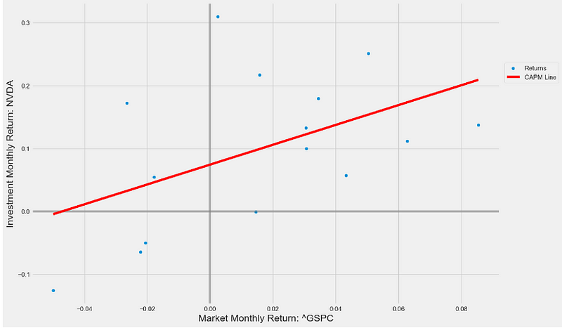
Examining the Market vs Investment Monthly Returns

stock_a =['NVDA']
stock_m = ['^GSPC']

CAPM(stock_a,stock_m,start, end)

========================================
Beta from formula:  1.5791
Beta from Linear Regression:  1.5791
Alpha:  0.074
========================================

CAPM Line for NVDA vs ^GSPC Monthly Returns

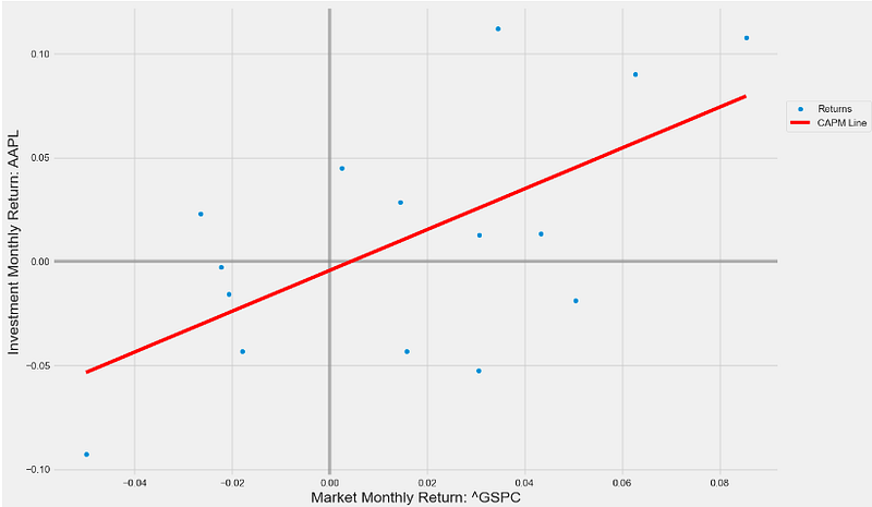
stock_a =['AAPL']
stock_m = ['^GSPC']

CAPM(stock_a,stock_m,start, end)

========================================
Beta from formula:  0.9823
Beta from Linear Regression:  0.9823
Alpha:  -0.004
========================================

CAPM Line for AAPL vs ^GSPC Monthly Returns

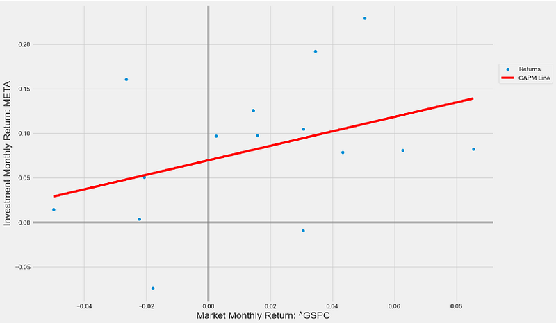
stock_a =['META']
stock_m = ['^GSPC']

CAPM(stock_a,stock_m,start, end)

========================================
Beta from formula:  0.8131
Beta from Linear Regression:  0.8131
Alpha:  0.07
========================================

CAPM Line for META vs ^GSPC Monthly Returns

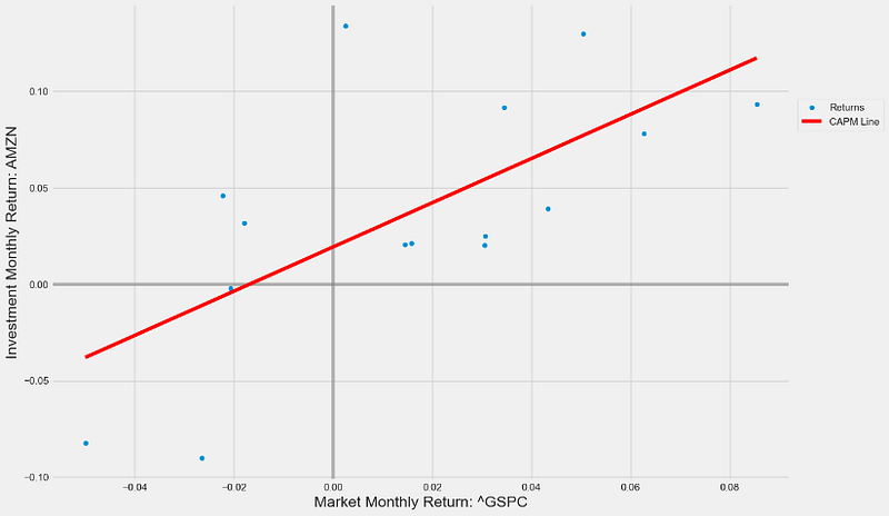
stock_a =['AMZN']
stock_m = ['^GSPC']

CAPM(stock_a,stock_m,start, end)

========================================
Beta from formula:  1.1471
Beta from Linear Regression:  1.1471
Alpha:  0.019
========================================

CAPM Line for AMZN vs ^GSPC Monthly Returns

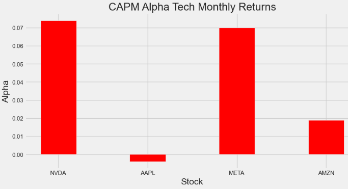
Creating a bar plot of the Estimated CAPM Alpha Tech Monthly Returns

# creating the dataset
data = {'NVDA':0.074, 'AAPL':-0.004, 'META':0.07, 
        'AMZN':0.019}
xvalues = list(data.keys())
yvalues = list(data.values())
  
fig = plt.figure(figsize = (10, 5))
 
# creating the bar plot
plt.bar(xvalues, yvalues, color ='red', 
        width = 0.4)
 
plt.xlabel("Stock")
plt.ylabel("Alpha")
plt.title("CAPM Alpha Tech Monthly Returns")
plt.show()

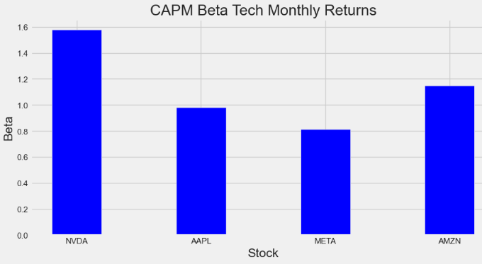
Creating a bar plot of the Estimated CAPM Beta Tech Monthly Returns

# creating the dataset
data = {'NVDA':1.5791, 'AAPL':0.9823, 'META':0.8131, 
        'AMZN':1.1471}
xvalues = list(data.keys())
yvalues = list(data.values())
  
fig = plt.figure(figsize = (10, 5))
 
# creating the bar plot
plt.bar(xvalues, yvalues, color ='blue', 
        width = 0.4)
 
plt.xlabel("Stock")
plt.ylabel("Beta")
plt.title("CAPM Beta Tech Monthly Returns")
plt.show()

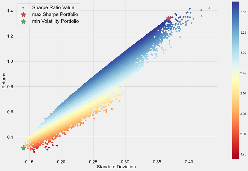
Max Sharpe Efficient Frontier

Let’s construct the Markowitz portfolio optimization model using the stochastic simulation algorithm. Our objective is to provide the highest Sharpe Ratio, which is a metric that compares the amount of return versus the amount of risk, based on historical data. Return is based on CAGR and risk is based on volatility. The portfolio is well suited for risk adverse investors with moderate growth expectations.
Creating max Sharpe and min Volatility Portfolios using simulated random portfolios

def calc_portfolio_perf(weights, mean_returns, cov, rf):
    portfolio_return = np.sum(mean_returns * weights) * 252
    portfolio_std = np.sqrt(np.dot(weights.T, np.dot(cov, weights))) * np.sqrt(252)
    sharpe_ratio = (portfolio_return - rf) / portfolio_std
    return portfolio_return, portfolio_std, sharpe_ratio
def simulate_random_portfolios(num_portfolios, mean_returns, cov, rf):
    results_matrix = np.zeros((len(mean_returns)+3, num_portfolios))
    for i in range(num_portfolios):
        weights = np.random.random(len(mean_returns))
        weights /= np.sum(weights)
        portfolio_return, portfolio_std, sharpe_ratio = calc_portfolio_perf(weights, mean_returns, cov, rf)
        results_matrix[0,i] = portfolio_return
        results_matrix[1,i] = portfolio_std
        results_matrix[2,i] = sharpe_ratio
        #iterate through the weight vector and add data to results array
        for j in range(len(weights)):
            results_matrix[j+3,i] = weights[j]
            
    results_df = pd.DataFrame(results_matrix.T,columns=['ret','stdev','sharpe'] + [ticker for ticker in tickers])
        
    return results_df

mean_returns = df.pct_change().mean()
cov = df.pct_change().cov()
num_portfolios = 100000
rf = 0.0
results_frame = simulate_random_portfolios(num_portfolios, mean_returns, cov, rf)

#locate position of portfolio with highest Sharpe Ratio
max_sharpe_port = results_frame.iloc[results_frame['sharpe'].idxmax()]
#locate positon of portfolio with minimum standard deviation
min_vol_port = results_frame.iloc[results_frame['stdev'].idxmin()]
plt.rc('font', size=14) 
#create scatter plot coloured by Sharpe Ratio
plt.subplots(figsize=(15,10))
plt.scatter(results_frame.stdev,results_frame.ret,c=results_frame.sharpe,cmap='RdYlBu')
plt.xlabel('Standard Deviation')
plt.ylabel('Returns')
plt.colorbar()
#plot red star to highlight position of portfolio with highest Sharpe Ratio
plt.scatter(max_sharpe_port[1],max_sharpe_port[0],marker=(5,1,0),color='r',s=500)
#plot green star to highlight position of minimum variance portfolio
plt.scatter(min_vol_port[1],min_vol_port[0],marker=(5,1,0),color='g',s=500)
plt.legend(["Sharpe Ratio Value","max Sharpe Portfolio" , "min Volatility Portfolio"],fontsize="18", loc ="upper left")
plt.yticks(fontsize=16)
plt.xticks(fontsize=16)
plt.show()

Simulated random portfolios, max Sharpe & min Volatility Portfolios

Comparing the 2 stock weighting tables that made up those two portfolios, along with the annualized return (ret), STDEV and Sharpe ratio, viz.

max_sharpe_port.to_frame().T

      ret      stdev   sharpe   SPY      AAPL     META     NVDA     AMZN
25825 1.338156 0.36815 3.634807 0.005907 0.028012 0.470447 0.480056 0.015578

min_vol_port.to_frame().T

      ret     stdev    sharpe   SPY      AAPL     META     NVDA     AMZN
57582 0.31199 0.140741 2.216772 0.710772 0.204089 0.012964 0.009955 0.06222

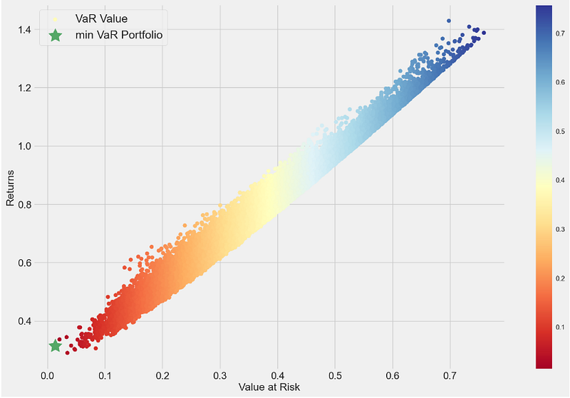
Min VaR Efficient Frontier

Identifying the portfolio weights that minimize the Value at Risk (VaR)

def calc_portfolio_perf_VaR(weights, mean_returns, cov, alpha, days):
    portfolio_return = np.sum(mean_returns * weights) * days
    portfolio_std = np.sqrt(np.dot(weights.T, np.dot(cov, weights))) * np.sqrt(days)
    portfolio_var = abs(portfolio_return - (portfolio_std * stats.norm.ppf(1 - alpha)))
    return portfolio_return, portfolio_std, portfolio_var

def simulate_random_portfolios_VaR(num_portfolios, mean_returns, cov, alpha, days):
    results_matrix = np.zeros((len(mean_returns)+3, num_portfolios))
    for i in range(num_portfolios):
        weights = np.random.random(len(mean_returns))
        weights /= np.sum(weights)
        portfolio_return, portfolio_std, portfolio_VaR = calc_portfolio_perf_VaR(weights, mean_returns, cov, alpha, days)
        results_matrix[0,i] = portfolio_return
        results_matrix[1,i] = portfolio_std
        results_matrix[2,i] = portfolio_VaR
        #iterate through the weight vector and add data to results array
        for j in range(len(weights)):
            results_matrix[j+3,i] = weights[j]
            
    results_df = pd.DataFrame(results_matrix.T,columns=['ret','stdev','VaR'] + [ticker for ticker in tickers])
        
    return results_df

mean_returns = df.pct_change().mean()
cov = df.pct_change().cov()
num_portfolios = 100000
rf = 0.0
days = 252
alpha = 0.05
results_frame = simulate_random_portfolios_VaR(num_portfolios, mean_returns, cov, alpha, days)

#locate positon of portfolio with minimum VaR
min_VaR_port = results_frame.iloc[results_frame['VaR'].idxmin()]
#create scatter plot coloured by VaR
plt.subplots(figsize=(15,10))
plt.scatter(results_frame.VaR,results_frame.ret,c=results_frame.VaR,cmap='RdYlBu')
plt.xlabel('Value at Risk')
plt.ylabel('Returns')



plt.colorbar()
#plot red star to highlight position of minimum VaR portfolio
plt.scatter(min_VaR_port[2],min_VaR_port[0],marker=(5,1,0),color='g',s=500)

plt.legend(["VaR Value","min VaR Portfolio"] ,fontsize="18", loc ="upper left")
plt.yticks(fontsize=16)
plt.xticks(fontsize=16)
plt.show()

Simulated random portfolios & min VaR Portfolio

The stock weighting table that made up the above portfolio is given by

min_VaR_port.to_frame().T

      ret      stdev    VaR     SPY      AAPL     META     NVDA     AMZN
20537 0.314227 0.182932 0.01333 0.159629 0.779188 0.017246 0.016846 0.027091

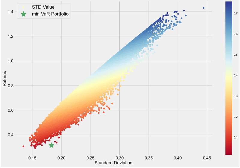
Finally, converting the horizontal axis from VaR to STDEV (cf. here)

#locate positon of portfolio with minimum VaR
min_VaR_port = results_frame.iloc[results_frame['VaR'].idxmin()]
#create scatter plot coloured by VaR
plt.subplots(figsize=(15,10))
plt.scatter(results_frame.stdev,results_frame.ret,c=results_frame.VaR,cmap='RdYlBu')
plt.xlabel('Standard Deviation')
plt.ylabel('Returns')
plt.colorbar()
#plot red star to highlight position of minimum VaR portfolio
plt.scatter(min_VaR_port[1],min_VaR_port[0],marker=(5,1,0),color='g',s=500)

plt.legend(["STD Value","min VaR Portfolio"] ,fontsize="18", loc ="upper left")
plt.yticks(fontsize=16)
plt.xticks(fontsize=16)

plt.show()

Simulated random portfolios & min VaR Portfolio in the Returns — STDEV plane

Conclusions

In this post, we have compared several popular stochastic portfolio optimization techniques that maximize returns while minimizing risk, excluding product costs and related fees.
It turns out that max Sharpe is the best tech portfolio in terms of the ret-to-stdev ratio

           minVaR    minVol    maxSharpe
ret   %    31        31        134
stdev %    18        14        37
ratio      1.72      2.21      3.62

We have compared the CAPM Lines of Monthly Returns for our stocks against the benchmark (^GSPC).
According to the estimated CAPM Alpha (Beta), a positive value of 0.074 (0.81) is good for NVDA (META) as compared to other 3 tech stocks.
Results confirm that NVDA and META remain our tech growth stocks in focus today, indicating bullish sentiments.

Portfolio Optimization of 4 Major Techs: Markowitz, Sharpe, VaR & CAPM

Business Case / Motivation

A Lean Environment Setup

Input Stock Data Analysis

Analysis of Log Returns

CAPM Line Alpha & Beta Monthly Returns

Max Sharpe Efficient Frontier

Min VaR Efficient Frontier

Conclusions

Explore More

References

Acknowledgements

Contacts