Harnessing the Power of Efficient Frontier and Max Sharpe Ratio for Risk Management of Day Trading with AI

As a day trading practitioner, I cannot emphasize more about risk management. A common belief is that risk management starts when you define your entry, target profit level, and stop loss level. In fact, it starts even before that. When you are encountered a series of actively traded stocks that are suitable for day trading every morning, you need to decide on picking the right stock to trade. Risk management has already started. A bad choice could induce all kinds of psychological pitfalls and a day of huge loss. That’s the first obstacle to overcome in risk management. For many day traders, that choice is very much discretionary and not optimized. On March 24, 2023, let’s say the following six actively traded stocks were identified suitable for day trading due to their volume and volatility in the premarket: FRC, BAC, TSLA, SQ, COIN, and ATVI. Which one or ones should you eventually pick to day trade given the following premarket OHLCV charts on a 5-min time frame?

This appears to be a problem without a definite right or wrong answer as everyone would give his or her preference. If you like low risk and low return, trading large-float stocks such as TSLA appears a good option. If you like high return, you could trade FRC and others, but the risks are much greater.

I would argue that there is a definite answer, and in this article, I’m going to introduce my method of extrapolating the financial concepts of efficient frontier and maximum Sharpe ratio that are commonly used in the investing field to the day trading field for finding the best stock(s) to trade. And yes, theoretically, there is only one answer that gives you the lowest risk per profit dollar — a scenario that every normal trader won’t decline. Knowing this answer with the help of AI will give you an edge to trade confidently. Please click “follow” if you haven’t done so and buckle up, we will get started!

The Theoretical Foundation

I have benefited a lot from the portfolio theory in course 15.401 Financial Theories taught by Professor Andrew Lo at MIT in 2008 (An open courseware that is available on YouTube) and two subsequent articles (authored by Gregory Gundersen Link 1 and Link 2) derived from it discussing the linear algebra involved in the computations. The portfolio theory basically says you need to diversify your portfolio in a specific way so that high expected return but low risk are achievable. If you have an option of risking 1 dollar to get 2 dollars and an option of risking 1 dollar to get 1 dollar, the portfolio theory assumes the former as the preference. In other words, you prefer to risk 0.5 dollar per 1 profit dollar than 1 dollar per 1 profit dollar. By doing so, your risk of investing or trading is reduced.

The portfolio theory presents a mean-variance method to find out the best weights of tickers based on which you should split your money for investing or trading. The best weights are dependent on your acceptable risk (return). For each acceptable risk (return), there is one and only one set of optimized weights. Plotting the risk (denoted as standard deviation of return) versus the mean return gives you the efficient frontier. The efficient frontier is the most northwestern line you can get for all possible combinations of weights. And we would love the line to be the most northwestern because that means on that line, we have the maximum return for a given risk, which is denoted by the Sharpe ratio — the normalized return by the risk with inclusion of a risk-free rate. On the efficient frontier curve, the Sharpe ratio is the maximum for any specified risk.

We might be still not satisfied with the efficient frontier, which gives the best return for a given risk. What about if we want the best return per risk? That would be the best of the best. To get that best-of-the-best point on the efficient frontier curve, we need to draw a tangent line starting from the risk-free rate to the bullet shape of the efficient frontier curve. The point where the tangent line and efficient frontier meets has the maximum Sharpe ratio, which gives the best of the best, as measured by the maximum return per risk or the lowest risk per return. That maximum Sharpe ratio point on the efficient frontier curve is what I would like to find out to guide my day trading so that based on the weight distribution I know what stock I should trade.

Assumptions for Extrapolating the Financial Theory to Day Trading

We will have to make the following three important assumptions to extrapolate the financial theory of efficient frontier and maximum Sharpe ratio to day trading:

1. The market is efficient. That means the stock prices walk randomly and there are no patterns to be employable by day traders, because if there is one, it must have been utilized by the smartest minds in the market and the pattern has gone. It is like the famous conversations between two economists walking on the street and decided not to pick up the $100 bill lying on the ground because if the bill is genuine, it must have been picked up by others. That’s the reason why the theory requires no prediction on the market move because it has assumed the market is efficient and there is no free lunch and no one can make easy money from the market. That’s the basis for the mean-variance relationship. For day trading, we rephrase this assumption this way: Because the stock prices walk randomly and there are no employable patterns, there is no need to predict the stock directions in day trading. With this assumption as the basis, we can select the best stocks to day trade using the mean-variance relationship derived from the historical prices.

2. For investment, it is assumed the market is on a generally rising trend despite of different kinds of pullbacks. So, our expected returns stay positive. Otherwise, who will invest in the market? For day trading, however, we know this cannot be true, because in our day trading timeframe we can either long or short stocks based on the beliefs of rising or falling trends. Therefore, we rephrase this assumption this way: it is assumed the day traders’ longing or shorting activities have a target for a positive return. This modified assumption makes our expected returns of day trading stay positive.

3. All stocks are uncorrelated. The financial theory states that you cannot find two stocks that are strictly inversely correlated (We don’t include the cheap answer of shorting the market here). However, you can find two positively correlated stocks, as many stocks move together with the market. As long as the correlation is neither 1 nor -1, the theory is valid for investing. For day trading, we also assume the correlations among the stocks are also neither 1 nor -1. If they are, you would do the opposite to take the free money, which cannot exist. This is the same analogy used in the justification of this assumption for using the efficient frontier theory for investing.

How the three assumptions affect our computations?

The first assumption on the price randomness ensures there is no need for prediction so that we can use the historical prices to derive the mean return and variance for each stock. If you don’t believe that, I have another article in my book Day Trade with AI discussing how to incorporate predictions into the mean return and variance computations for each stock. So, stay tuned! For now, let’s stick to this assumption and compute the price fluctuations in the premarket for each 5-min OHLC candle. We then compute the standard deviation of these price fluctuations, which will be used in the mean-variance relationship.

The second assumption on the positive expected returns validates the application of both longing and shorting activities in day trading. For each 5-min OHLC candle, we will use the absolute value of the spread of high and low prices as the expected return for the computation of the mean return, because we can do whatever longing or shorting to achieve the goal of a positive expected return. You will have to believe that, because if you don’t, well, why do you (learn to) day trade if your expected return is negative? Unfortunately, this is a reason why people quit day trading, because from their negative return experiences in day trading, they see no future of getting a positive return. If you are doubtful on this assumption, you should not day trade in the first place.

The third assumption on the uncorrelation ensures the existence of the efficient frontier. In fact, we know even if the stocks in the same sector tended to move together in the same direction, when we examine the price actions tick by tick, they are not exactly in the same direction in that respective. In this demonstration, the stocks are picked from a list with a criteria of high pre-market volume and volatility, it is less likely that they come from the same sector, and most importantly, we trade in a short time frame. So, the directions in that 5-min time frame can be uncorrelated. Note that if the third assumption fails, which could happen, neither the investing nor trading has a valid efficient frontier anymore, and all financial theories fail. An example for investing would be the 2008 stock market crash. An example for trading would be having SVB (The Silicon Valley Bank) and FRC (First Republic Bank) who were both driven under the same bankruptcy crisis.

Great! After I clear out the three most important assumptions, the efficient frontier and maximum Sharpe ratio theory can be fully extrapolated to day trading practices. Let’s do the coding part to find out the best stock(s) to trade and their weights in reducing your risk while maximizing your profits!

Code Implementation

We will need the following libraries to get started. In addition to the common datetime module and the Pandas, NumPy, and Matplotlib libraries, we need finnhub to download the premarket OHLCV data for each stock, seaborn to generate the covariance matrix, and SciPy to do the optimization work. The documentation for finnhub is here, where you need to apply for a free API key to run the code.

import datetime as dt
import finnhub
import pandas as pd
import numpy as np
import matplotlib.pyplot as plt
import seaborn as sns
from scipy.optimize import minimize

finnhub_api_key = 'REPLACE THIS WITH YOUR KEY' # replace this with your key
tickers = ['FRC','BAC','TSLA','SQ','COIN','ATVI']
start = dt.datetime(2023,3,24,0,0,0)
end = dt.datetime(2023,3,24,9,29,0)

def get_5m_data(ticker,start,end,finnhub_api_key):
    finnhub_client = finnhub.Client(api_key=finnhub_api_key)
    res = finnhub_client.stock_candles(ticker, '5', int(start.timestamp()), int(end.timestamp()))
    df = pd.DataFrame(res)
    df['t'] = [dt.datetime.fromtimestamp(df['t'][ind]) for ind,_ in df.iterrows()]
    df.set_index('t',inplace=True)
    df = df[['o','h','l','c','v']]
    return df

df_di = {}
for ticker in tickers:
    df_di[ticker] = get_5m_data(ticker,start,end,finnhub_api_key)

Make sure you replace the finnhub_api_key with your key if you want to implement the code by yourself. As you can see, I downloaded the 5-min timeframe premarket data for each ticker from the list of FRC, BAC, TSLA, SQ, COIN, and ATVI for March 24, 2023, and then stored them into the dataframe dictionary called df_di.

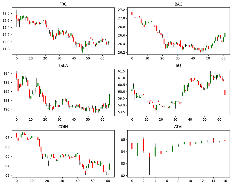
I used the following code to visualize the 6 dataframes in the dataframe dictionary.

# Visualize the 6 tickers
plt.figure(figsize=(10,8))

for i,ticker in enumerate(tickers):
    plt.subplot(3,2,i+1)
    j = 0
    for ind in df_di[ticker].index:
        plt.vlines(x = j, ymin = df_di[ticker].loc[ind,'l'], ymax = df_di[ticker].loc[ind,'h'], color = 'black', linewidth = 1)     
        if df_di[ticker].loc[ind,'o'] > df_di[ticker].loc[ind,'c']:
            plt.vlines(x = j, ymin = df_di[ticker].loc[ind,'c'], ymax = df_di[ticker].loc[ind,'o'], color = 'red', linewidth = 3)        
        elif df_di[ticker].loc[ind,'o'] < df_di[ticker].loc[ind,'c']:
            plt.vlines(x = j, ymin = df_di[ticker].loc[ind,'o'], ymax = df_di[ticker].loc[ind,'c'], color = 'green', linewidth = 3)              
        else:
            plt.vlines(x = j, ymin = df_di[ticker].loc[ind,'o'], ymax = df_di[ticker].loc[ind,'c'], color = 'black', linewidth = 3)
        j += 1
    plt.title(ticker)
    plt.tight_layout()

As you can see, their patterns are not the same, so the correlations should neither be 1 or -1 (We can confirm this later when computing the covariance matrix). This ensures we have an efficient frontier!

When computing the mean and variances (or the standard deviation), I only picked the 5-min OHLC data after 7 am in the premarket, because it is my experience that only after 7 am the real move that can be employed by day traders might occur. The reason I computed the mean 5-min return is that it is my preferred trading style of holding a stock for a duration as short as 5 minutes. Feel free to tweak these numbers to fit your trading style if you wish.

index_start_time = dt.datetime(start.year,start.month,start.day,7,0,0)
full_index = pd.date_range(index_start_time, periods=30, freq='5min')
df = pd.DataFrame(index=full_index, columns=tickers)

I pivoted the 6 dataframes into one single dataframe with the values of computed expected returns within 5 minutes measured by the absolute value of the spread of high and low in each 5-min OHLC candle.

for ticker in tickers:
    for i,r in df.iterrows():
        if i in df_di[ticker].index:
            if df_di[ticker].loc[i,'c'] >= df_di[ticker].loc[i,'o']:
                df.loc[i,ticker] = (df_di[ticker].loc[i,'h']-df_di[ticker].loc[i,'l'])/df_di[ticker].loc[i,'l']*100
            else:
                df.loc[i,ticker] = (df_di[ticker].loc[i,'l']-df_di[ticker].loc[i,'h'])/df_di[ticker].loc[i,'h']*100

ret,std= np.zeros((len(tickers),1)),np.zeros((len(tickers),1))
for i in range(len(tickers)):
    ret[i,0] = abs(df.iloc[:,i]).mean()
    std[i,0] = df.iloc[:,i].std()
df = df.fillna(0)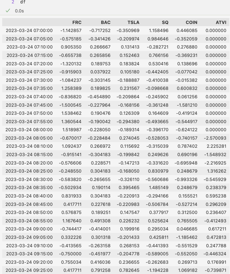

The dataframe is further visualized by a heatmap for the illustration of the correlations. As you can see, none of the off-diagonal blocks had values of 1 or -1, confirming that the efficient frontier exists!

sns.heatmap(df.corr(),annot=True)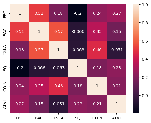

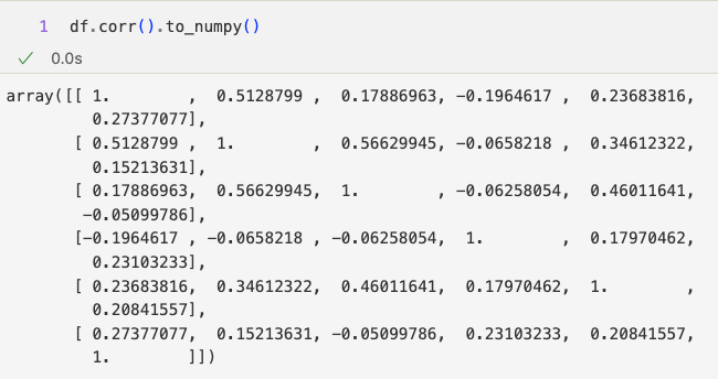
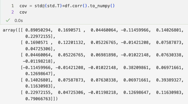
The correlations are converted to the covariance matrix by element-wise multiplication of the standard deviation matrix with the correlation matrix.

df.corr().to_numpy()

cov = std@(std.T)*df.corr().to_numpy()
cov

With the computed mean return and standard deviation for each stock, we can plot these numbers on the graph as follows. It clearly shows that FRC has the highest return and the highest risk. TSLA has the lowest return and the lowest risk. The other 4 stocks are in the middle. This may sound common sense to most experienced traders. Well, this is just a check to make sure we are not producing something nonsense. And for beginning traders and those who feel their brains are under high pressure while trading, this chart can help them to quantitatively screening the to-be-traded stock list based on their preferred expected return or risk level.

plt.scatter(std,ret)
for i in range(len(tickers)):
    plt.text(std[i,0]+0.02,ret[i,0],tickers[i])
plt.xlabel('Standard Deviation of Returns')
plt.ylabel('Expectation of Returns')
plt.show()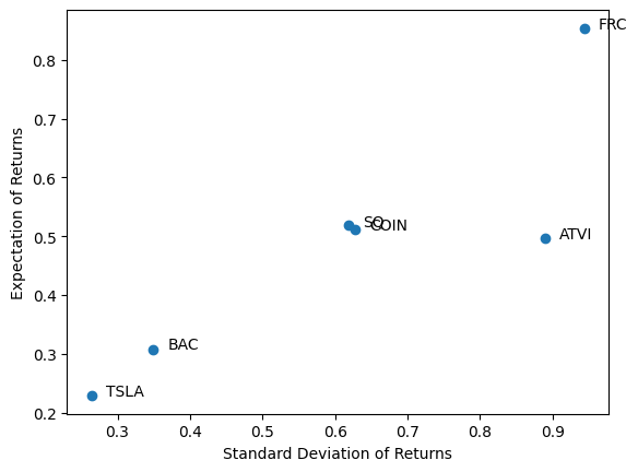

Now, next is the most exciting part! We will produce the efficient frontier using these 6 tickers and the best-of-the-best portfolio constructed using these 6 tickers you should consider holding for 5 minutes whenever you feel a good timing.

def portfolio_performance(ret,cov,w):
    ret_p = w.T@ret
    std_p = np.sqrt(w.T@cov@w)
    return ret_p,std_p

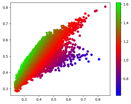
# Find efficient frontier via sampling.
x = np.empty(5000)
y = np.empty(5000)
for i in range(5000):
    w = np.random.dirichlet([1]*len(tickers)).reshape(len(tickers),1)
    y[i], x[i] = portfolio_performance(ret, cov, w)
s = y/x #sharpe ratio with risk-free rate of 0
sn = s/(s.max()-s.min())
plt.scatter(x, y, c=sn, cmap='brg')
plt.colorbar()

In this code block, a function is defined to compute a portfolio’s expected return and standard deviation of the return. Then we randomly sample 5000 sets of weights while making sure the sum of each set of weights sums to 1. For each set of weights, the portfolio’s expected return and standard deviation are computed and recorded as y and x, respectively. The Sharpe ratio for each portfolio is also computed by assuming a risk-free rate of zero. This makes sense because if you don’t trade, the risk is zero. There is no risk-free bond in the realm of day trading that gives you some kind of positive number of returns. We then visualize the sampled data colored by the normalized Sharpe ratios. More northwestern, higher the Sharpe ratio!

Now we need to find the efficient frontier that gives use the best return with a specified risk. Here we use the SciPy’s minimize function. Feeding the function with a list of target returns from 0.2 to 1% (stored in yy), it finds the minimal risk (stored in xx) and weights (stored in w_li) for each target return. Plotting xx versus yy gives us the efficient frontier! As long as you trade the six stocks with the weights on that efficient frontier, you can’t get any better with a specified risk! Fantastic!

# Find efficient frontier numerically.
def efficient_portfolio(targ,ret,cov,w,tickers):
    def objective(w):
        return w.T @ cov @ w - targ * w.T @ ret
    resp = minimize(objective,
                    x0=np.random.dirichlet([1]*len(tickers)),
                    method='SLSQP',
                    bounds=[(-2, 2)]*len(tickers),
                    constraints=[
                        {'type': 'eq', 'fun': lambda w: 1 - w.sum()},
                        {'type': 'eq', 'fun': lambda w: w.T@ret - targ}
                    ])
    return resp.x

xx = np.empty(100)
yy = np.empty(100)
w_li = []

for i, targ in enumerate(np.linspace(0.2, 1, 100)):
    w = efficient_portfolio(targ,ret,cov,w,tickers)
    yy[i], xx[i] = portfolio_performance(ret, cov, w)
    w_li.append(w)

plt.plot(xx, yy)
plt.xlabel('Standard Deviation of Returns')
plt.ylabel('Expectation of Returns')
plt.show()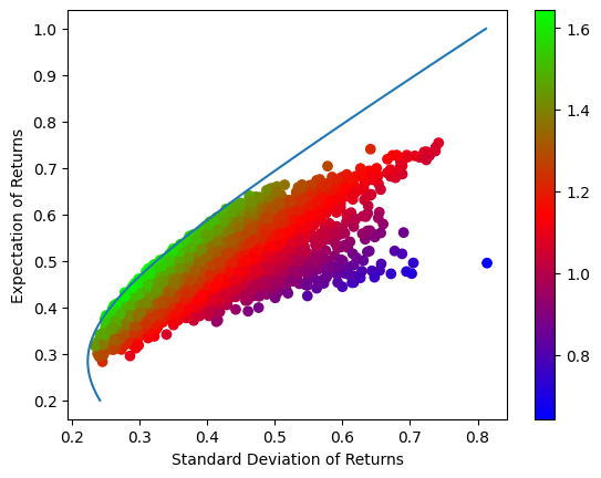

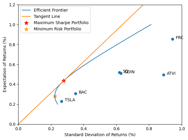
Now what about the best of the best? That is based on the computation of Sharpe ratios on the efficient frontier curve. As you can see, there is a highest Sharpe ratio we can find in the list of our computed ratios on the efficient frontier. The index of that highest value will get us to the best-of-the-best portfolio for day trading.

sr = yy/xx # sharpe ratio with risk-free rate of 0
plt.plot(range(len(sr)),sr)
plt.xlabel('Indices of Sharpe Ratio in the Computed List')
plt.ylabel('Sharpe Ratio')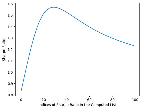

While using a line connecting zero and the best-of-the-best point on the efficient frontier, we find this line is the tangent line! All computations are verified!

plt.plot(xx, yy,label='Efficient Frontier')
plt.scatter(std,ret)
plt.plot(np.linspace(0,0.8,100),np.linspace(0,0.8,100)*yy[sr.argmax()]/xx[sr.argmax()],label='Tangent Line')
plt.scatter(xx[sr.argmax()],yy[sr.argmax()],s=100,marker='*',c='red',label='Maximum Sharpe Portfolio')
plt.scatter(xx[xx.argmin()],yy[xx.argmin()],s=100,marker='*',c='orange',label='Minimum Risk Portfolio')

for i in range(len(tickers)):
    plt.text(std[i]+0.02,ret[i],tickers[i])
plt.xlabel('Standard Deviation of Returns (%)')
plt.ylabel('Expectation of Returns (%)')
plt.xlim([0,1])
plt.ylim([0,1.2])
plt.legend()
plt.tight_layout()
plt.show()

Interpretations and Concluding Remarks

What can we get from here? How can this result guide us in day trading? Let’s print out the weights of two portfolios for day trading: one for the maximum Sharpe portfolio, and the other for the minimum risk portfolio, and discuss the implications.

print(f'Maximum Sharpe Portfolio (Tangency Portfoio) with a return of {yy[sr.argmax()]:.2f}% and a standard deviation of {xx[sr.argmax()]:.2f}%')
for weight, ticker in zip(w_li[sr.argmax()],tickers):
    print(ticker, weight)

print(f'\nMinimum Risk Portfolio with a return of {yy[xx.argmin()]:.2f}% and a standard deviation of {xx[xx.argmin()]:.2f}%')
for weight, ticker in zip(w_li[xx.argmin()],tickers):
    print(ticker, weight)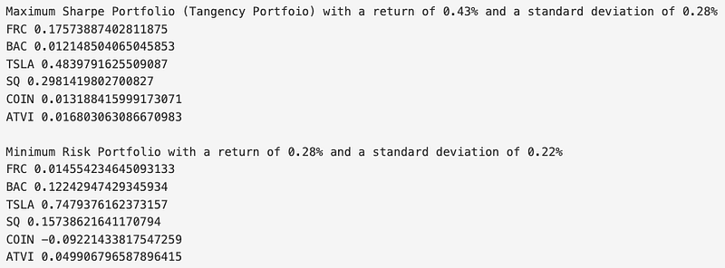

As you can see, the maximum Sharpe portfolio suggest you mainly trade TSLA (0.48), SQ (0.30), and FRC (0.18) to get an expected return of 0.43% with a standard deviation of 0.28% by trading my style of holding the stocks for 5 minutes. On the other hand, the minimum risk portfolio suggest you mainly trade TSLA (0.75), SQ (0.16), and BAC (0.12) to get an expected return of 0.28% with a standard deviation of 0.22% by momentum trading in my style. Is this result helpful? It is definitely helpful for me, because the computer had done the complicated work and directly present me with the optimized results, which save a lot of my brain power that can be put into other applications such as scrutinizing the emotions in the market in the highly stressful day trading practices. I hope you feel the same too.

The result also has a potential to guide automated algorithmic trading, which can accurately split the fund to trade different stocks in a very short period of time.

You might see negative numbers in the recommended weights. For investing, the negative weight mean you should short the stock. However, for day trading, we have assumed we can use either longing or shorting activities to ensure the expected returns to be positive for extrapolation of this financial theory. So, the negative weight does not mean shorting here. It means you trade opposite to your strategy.

As I stressed earlier, the validity of the efficient frontier and maximum Sharpe ratio theory for day trading is contingent on three aforementioned assumptions. My book Day Trade with AI has the content to deal with the scenarios when these assumptions do not hold, as we are going to employ AI to predict the expected returns and the risks since we don’t believe the market is at randomness, do we? If we do, then we day traders are gamblers. Obviously, we are not, because we are the important component of the market that helps the market to become efficient. In other words, we are trained to have an edge to take the $100 bill from the ground before the two economists notice it. Stay tuned for my next article and make sure you have followed me and signed up the mail list when my book Day Trade with AI becomes available.

Disclaimer:

I do not make any guarantee or other promise as to any results that are contained within this article. You should never make any investment decision without first consulting with your financial advisor and conducting your own research and due diligence. To the maximum extent permitted by law, I disclaim any implied warranties of merchantability and liability in the event any information contained in this article proves to be inaccurate, incomplete, or unreliable or results in any investment or other losses.

I hope you enjoy reading the article. I periodically publish articles of original content on the applications of machine learning and deep learning in the realms of quantitative trading, finance, and engineering. I’m also writing my book Day Trade with AI, which is to be released soon. If you finish reading here and would like to see more of my writings, please follow me on Medium (https://shunyutang.medium.com/) or Twitter (https://twitter.com/shunyutang).

To support me, you can buy me a coffee by clicking here. I drink a lot of coffee while writing!

Subscribe to DDIntel Here.

Visit our website here: https://www.datadriveninvestor.com

Join our network here: https://datadriveninvestor.com/collaborate