The provided content outlines a comprehensive analysis of a risk-adjusted portfolio optimization strategy involving Bitcoin, Gold, Oil, and EUR/USD, utilizing advanced quantitative trading techniques and statistical models to maximize the risk-adjusted return.
Abstract
The article delves into a sophisticated quantitative approach for optimizing a portfolio that includes Bitcoin (BTC), Gold, Crude Oil, and the EUR/USD exchange rate. It employs a range of statistical and machine learning techniques, including AutoEDA, Scipy SLSQP, Markowitz's portfolio theory, and the Sharpe ratio, to construct a portfolio that aims to maximize the return-to-risk ratio. The study investigates the interconnectedness of these financial assets and their potential as hedge and safe-haven assets against stock market volatility. It also discusses the methodology for importing packages, performing automated EDA reports, handling missing data, converting currencies, and plotting log returns. The analysis includes time series analysis, such as ACF/PACF, ADF tests, and the fitting of ARIMA models, to ensure the stationarity of the data. The article further explores the use of Monte Carlo simulations to visualize the efficient frontier and the application of the Scipy SLSQP optimization algorithm to determine the optimal portfolio weights. The final comparison includes the efficient frontier, the tangency portfolio, and the minimum variance portfolio, with conclusions drawn on the diversification capabilities and risk-adjusted performance of the proposed portfolio.
Opinions
The article suggests that Bitcoin, despite its high volatility, can be part of a diversified investment portfolio that seeks to maximize risk-adjusted returns.
Gold is considered to have a low risk and is seen as a traditional safe-haven asset, while oil is recognized for its high volatility and lower return.
The study posits that a well-diversified portfolio can be constructed using quantitative methods to balance risk and return effectively.
The authors express that the Sharpe ratio is a critical metric for evaluating the performance of a portfolio, with a higher Sharpe ratio indicating a more favorable risk-adjusted return.
The use of advanced statistical models, such as ARIMA and GARCH, is advocated for understanding and predicting the behavior of financial time series data.
The Monte Carlo simulation is presented as a valuable tool for visualizing the range of possible outcomes and for identifying the efficient frontier in portfolio optimization.
The article concludes that the maximum Sharpe ratio portfolio may not always align with investor expectations, emphasizing the importance of considering additional risk metrics and investment strategies.
Risk-Adjusted BTC-Gold-Oil- EURUSD Portfolio Optimization for Quant Traders: AutoEDA, Scipy SLSQP, Markowitz, Sharpe & VAR
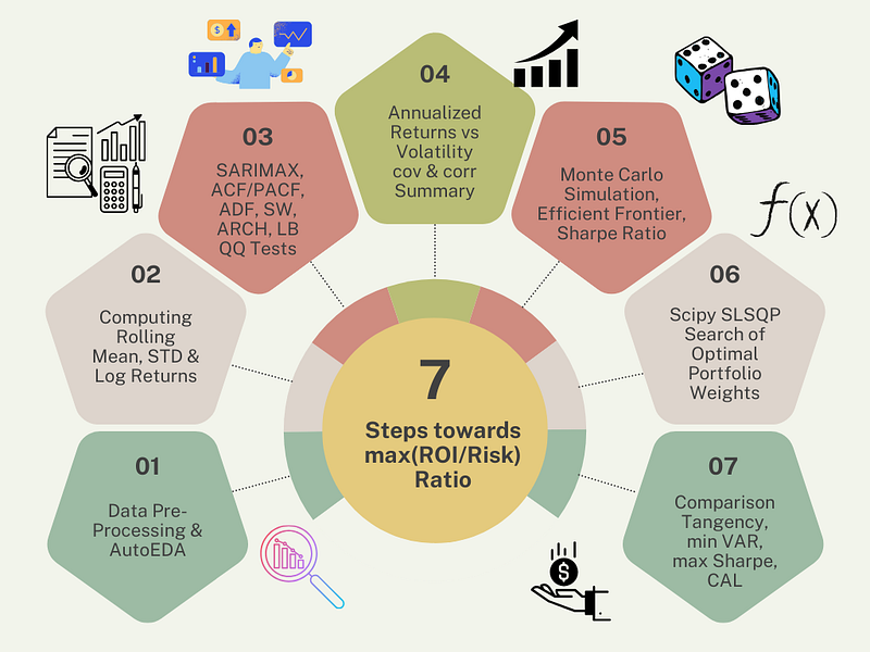
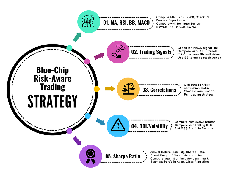
Risk-Adjusted Quant Trading Roadmap: 7 Steps towards max(ROI/Risk) or min(Risk/ROI)=min(Risk)/max(ROI) Ratio (image template via Canva).Investment Strategies for Beginners (image template via Canva).
Referring to the recent case example of fintech Time Series Analysis (TSA), this article investigates statistically significant relationships between Gold (GC=F), Crude Oil (CL=F), and Bitcoin (BTC) within the confines of risk-adjusted quant trading that maximizes the ROI/Volatility ratio.
Specifically, we model the linkages between BTC, gold, EUR, and crude oil using the stochastic portfolio optimization approach.
Our analysis also includes the EURUSD exchange rate risk. It accounts for the exposure faced by investors that operate across different countries within EU.
Goals
This study investigates whether gold, EUR/USD, oil and BTC are hedge and safe haven assets against stock and if they are useful in diversifying downside risk for international stock markets.
This is a financial adventure through time. It started around the 1950s with a financial wizard named Harry Markowitz (efficient frontier, max Sharpe ratio, min variance, CAL, etc.).
Key Task: download real-time stock data using yfinance to practice TSA (arch, scipy, statsmodels, etc.), GARCH model of residuals, ACF/PACF and Q-Q plot diagnostics, statistical testing (SARIMAX, ADF, Shapiro-Wilks, etc.), model estimation (AIC, BIC, etc.), and MPT in Python.
Motivation
BTC has attracted great attention around the world since its introduction in 2008.
But how has BTC performed against other asset classes such as precious metals and oil more recently?
Research indicates that BTC has the potential to replace gold as a hedge against inflation and become a new investment asset, with a strong substitution effect between the two assets.
The paper’s motivation is based upon the idea that BTC can be similar to gold in terms of its hedging properties and can be used for hedging for different assets. Moreover, although it is more metaphorical, BTC is also accepted because it is mined like crude oil, viz. a commodity. These similarities can be investigated by analyzing the connectedness among these financial assets in the sequel.
Scope
The proposed Risk-Adjusted Quant Trading Roadmap consists of the following 7 Steps geared towards max(ROI/Risk) Ratio:
Step 1: Input data loading, editing, pre-processing and Automated Exploratory Data Analysis (Auto EDA) with ydata-profiling & sweetviz.
Step 2: Computing rolling mean, std, and log daily returns of our assets.
Step 3: Analyzing ACF/PACF, ADF, checking the mean, skewness and kurtosis of log returns.
Step 4: Examining the SARIMAX statistical summary and residual plots (Q-Q, ACF, etc.), calculating annualized returns vs volatility, and comparing covariance vs correlations.
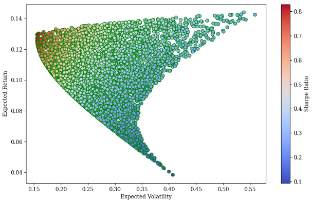
Step 5: Monte Carlo simulation of random portfolios, plotting the Markowitz efficient frontier vs the Sharpe ratio.
Step 6: Stochastic optimization of portfolio weights using the Scipy SLSQP method.
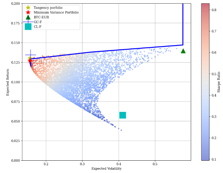
Step 7: Final comparison of the risk-adjusted portfolio against the efficient frontier, minimum variance and tangency portfolios that offer the highest expected return for a specific level of risk.
Let’s delve into details of this approach implemented in Python 3.12.2.
Importing Packages
Setting the working directory and importing packages
import os
os.chdir('YOURPATH') # Set the working directory
os. getcwd()
# Import packagesimport pandas as pd
import numpy as np
import matplotlib.pyplot as plt
import statsmodels.graphics.tsaplots as sgt
import statsmodels.tsa.stattools as sts
from statsmodels.tsa.arima_model import ARIMA, ARMA
import statsmodels.api as sm
import statsmodels.tsa.arima_model
from scipy import stats
from math import sqrt
import seaborn as sns
import pylab
import scipy
import yfinance
from arch import arch_model
from scipy.stats import shapiro
from statsmodels.stats.diagnostic import het_arch, acorr_ljungbox
#Basic Imports for Optimization import math
import scipy.stats as scs
import statsmodels.api as sm
from pylab import mpl, plt
import scipy.optimize as sco
import scipy.interpolate as sci
mpl.rcParams['font.family'] = 'serif'
%matplotlib inline
#AutoEDA
!pip install pandas_profiling, sweetviz
from pandas_profiling import ProfileReport
import sweetviz as sv
# to ignore some warnings in python when fitting models ARMA or ARIMAimport warnings
warnings.filterwarnings('ignore')
Reading Input Stock Data
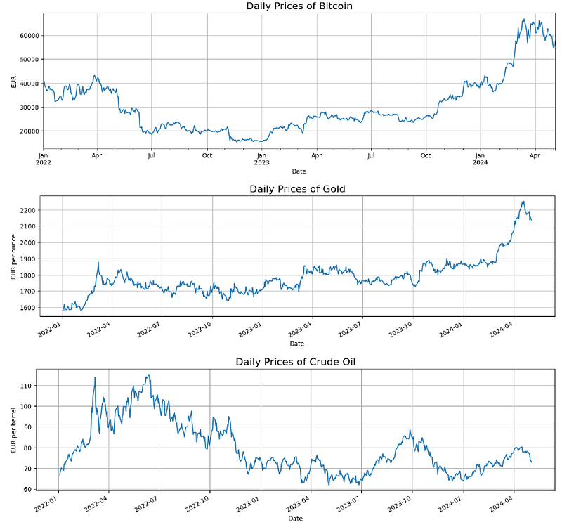
Reading the Adj Close of BTC-USD, GC=F, CL=F, and EURUSD=X from 2022–01–03 to 2024–05–03
# Bitcoin prices
df1.btc.plot(figsize=(15,4))
plt.ylabel("EUR")
plt.title('Daily Prices of Bitcoin', fontsize=16)
plt.grid()
plt.show()

# Gold prices
df2.gold.plot(figsize=(15,4))
plt.ylabel("EUR per ounce")
plt.title('Daily Prices of Gold', fontsize=16)
plt.grid()
plt.show()

# Oil prices
df3.oil.plot(figsize=(15,4))
plt.ylabel("EUR per barrel")
plt.title('Daily Prices of Crude Oil', fontsize=16)
plt.grid()
plt.show()
Daily prices of BTC, Gold and Oil
Rolling Mean & STD
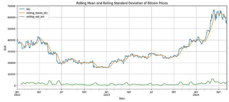
Calculating and plotting the rolling mean and STD of daily prices
df1['rolling_mean_btc'] = df1.btc.rolling(window=12).mean()
df1['rolling_std_btc'] = df1.btc.rolling(window=12).std()
df1.plot(title='Rolling Mean and Rolling Standard Deviation of Bitcoin Prices',
         figsize=(15,6))
plt.ylabel("EUR")
plt.grid()
plt.show()
Rolling Mean and Rolling Standard Deviation of Bitcoin Prices
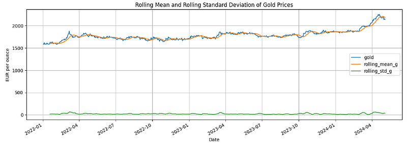
df2['rolling_mean_g'] = df2.gold.rolling(window=12).mean()
df2['rolling_std_g'] = df2.gold.rolling(window=12).std()
df2.plot(title='Rolling Mean and Rolling Standard Deviation of Gold Prices',figsize=(15,5))
plt.ylabel('EUR per ounce')
plt.grid()
plt.show()
Rolling Mean and Rolling Standard Deviation of Gold Prices
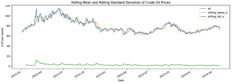
df3['rolling_mean_o'] = df3.oil.rolling(window=12).mean()
df3['rolling_std_o'] = df3.oil.rolling(window=12).std()
df3.plot(title='Rolling Mean and Rolling Standard Deviation of Crude Oil Prices',
         figsize=(15,5))
plt.ylabel('EUR per barrel')
plt.show()
Rolling Mean and Rolling Standard Deviation of Crude Oil Prices
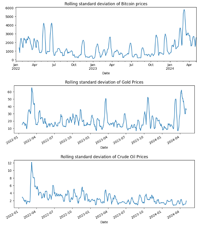
Plotting STD separately
df1['rolling_std_btc'].plot(title='Rolling standard deviation of Bitcoin prices', figsize=(10,3))
plt.show()
df2['rolling_std_g'].plot(title='Rolling standard deviation of Gold Prices', figsize=(10,3))
plt.show()
df3['rolling_std_o'].plot(title='Rolling standard deviation of Crude Oil Prices', figsize=(10,3))
plt.show()
Rolling standard deviation of BTC, Gold and Oil Daily Prices
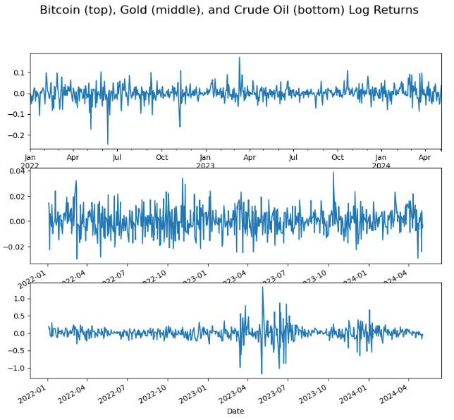
Log Returns
Calculating log returns of BTC, Gold and Oil Daily Prices in EUR
df1['log_ret_btc'] = np.log(df1.btc/df1.btc.shift(1))
df2['log_ret_g'] = np.log(df2.gold/df2.gold.shift(1))
#Handling negative values
df3['trans_o'] = df3['oil'] + 1 - df3['oil'].min()
df3['log_ret_o'] = np.log(df3.trans_o/df3.trans_o.shift(1))
# Check the missing values of the seriesprint('Number of missing values of Bitcoin log returns:', df1.log_ret_btc.isna().sum())
print('Number of missing values of Gold log returns:', df2.log_ret_g.isna().sum())
print('Number of missing values of Crude oil log returns:', df3.log_ret_o.isna().sum())
# Plot 3 series of log returns
fig, ax = plt.subplots(3, 1, figsize=(10,9))
df1.log_ret_btc.plot(ax=ax[0])
df2.log_ret_g.plot(ax=ax[1])
df3.log_ret_o.plot(ax=ax[2])
fig.suptitle('Bitcoin (top), Gold (middle), and Crude Oil (bottom) Log Returns', fontsize=16)
Log returns of BTC, Gold and Oil Daily Prices in EUR
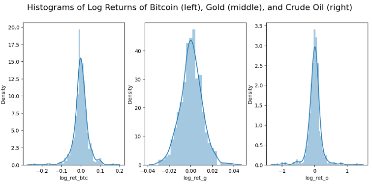
Plotting histograms of log returns
# Check the distribution of each series by histograms
fig, ax = plt.subplots(1, 3, figsize=(12,5))
sns.distplot(df1.log_ret_btc[1:], ax=ax[0])
sns.distplot(df2.log_ret_g[1:], ax=ax[1])
sns.distplot(df3.log_ret_o[1:], ax=ax[2])
fig.suptitle('Histograms of Log Returns of Bitcoin (left), Gold (middle), and Crude Oil (right)', fontsize=16)
plt.show()
Histograms of Log Returns of Bitcoin (left), Gold (middle), and Crude Oil (right)
Calculating the mean, skewness and kurtosis of these three distributions
The small positive mean return of each asset that the prices slightly increased over the period in general.
We can see that skewness(BTC)
0The positive skewness of a distribution indicates that an investor may expect frequent small losses and a few large gains from the investment.
Kurtosis(Gold)=0.6<
ACF & PACF Analysis
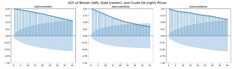
Plotting ACF of Bitcoin (left), Gold (center), and Crude Oil (right) Prices
# ACF
fig, ax = plt.subplots(1, 3, figsize=(20,5))
# Omit the lag 0
sgt.plot_acf(df1.btc, lags=40, zero=False, ax=ax[0])
sgt.plot_acf(df2.gold, lags=40, zero=False, ax=ax[1])
sgt.plot_acf(df3.oil, lags=40, zero=False, ax=ax[2])
fig.suptitle('ACF of Bitcoin (left), Gold (center), and Crude Oil (right) Prices', fontsize=16)
plt.show()
ACF of Bitcoin (left), Gold (center), and Crude Oil (right) Prices
We can see a strong correlation of prices at most lags. Therefore, the time series are not random.
In other words, the these time series are non-stationary since all lags are significant (lie outside of blue areas) and gradually decrease.
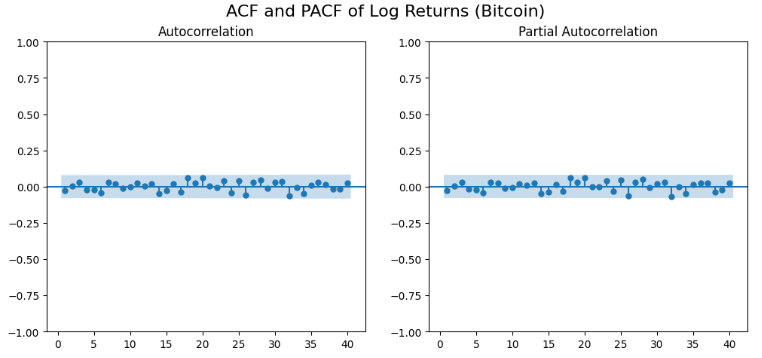
Plotting ACF/PACF of log returns
fig, ax = plt.subplots(1, 2, figsize=(12,5))
# Omit the lag 0
sgt.plot_acf(df1.log_ret_btc[1:], lags=40, zero=False, ax=ax[0])
sgt.plot_pacf(df1.log_ret_btc[1:], lags=40, zero=False, method=('ols'), ax=ax[1])
fig.suptitle('ACF and PACF of Log Returns (Bitcoin)', fontsize=16)
plt.show()
ACF and PACF of Log Returns (Bitcoin)
The ACF/PACF of the BTC log returns shows that there is only one autocorrelation that is significantly non-zero at a lag of 0. Therefore, the time series is random.
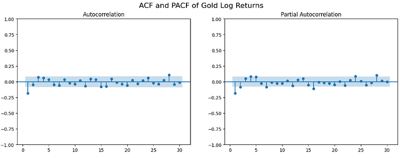
#Gold Log Returns
fig, ax = plt.subplots(1, 2, figsize=(15,5))
# Omit the lag 0
sgt.plot_acf(df2['log_ret_g'][1:], lags=30, zero=False, ax=ax[0])
sgt.plot_pacf(df2['log_ret_g'][1:], lags=30, zero=False, method=('ols'), ax=ax[1])
fig.suptitle('ACF and PACF of Gold Log Returns', fontsize=16)
plt.show()
ACF and PACF of Gold Log Returns
The ACF/PACF of the Gold log returns shows that there are a few autocorrelation values that are significantly non-zero. Therefore, the time series is not random.
ADF Test
Utilizing the Augmented Dickey–Fuller (ADF) test to determine the stationarity of daily prices
This test shows that p-value << 0.05 for all three log returns. A very low p-value of ADF tells that the null hypothesis of the test is very unlikely to be correct. In the ADF test, it would mean the tested series is stationary.
SARIMAX Summary
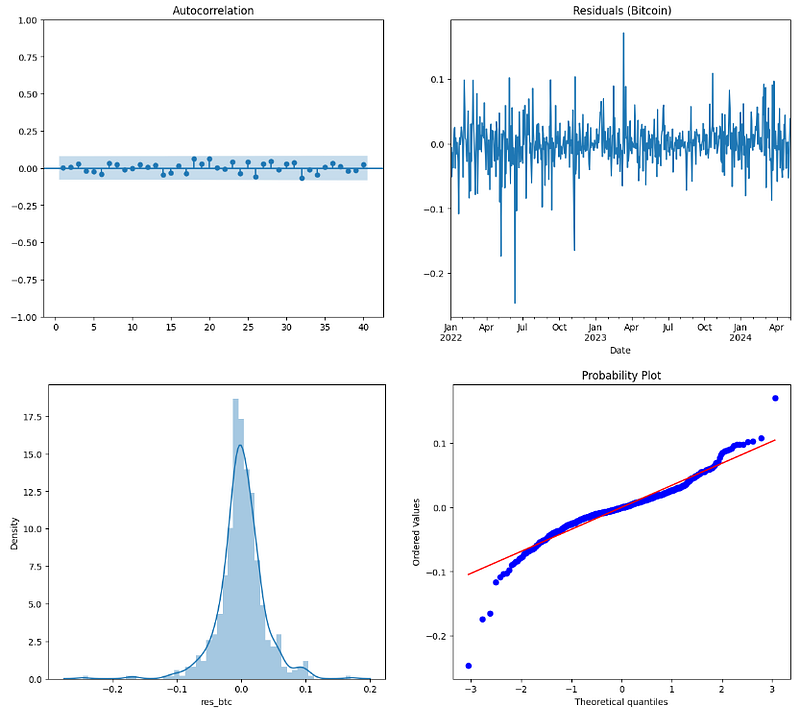
Fitting the possible ARIMA models for BTC log returns
# create residual series
df1['res_btc'] = results_btc_arima.resid
Examining the BTC residuals, ACF, histogram/density and Q-Q plot
fig, ax = plt.subplots(1, 2, figsize=(15,6))
# ACF of the residuals
sgt.plot_acf(df1.res_btc[1:], lags=40, zero=False, ax=ax[0])
# Plot the residuals
df1.res_btc.plot(title=" Residuals (Bitcoin)", ax=ax[1])
plt.show()

fig, ax = plt.subplots(1, 2, figsize=(15,6))
# Histogram of the estimated residuals
sns.distplot(df1.res_btc[1:], ax=ax[0])
# QQ-plot of the estimated residuals
scipy.stats.probplot(df1.res_btc[1:], plot=pylab)
pylab.show()
ACF, residuals, density and Q-Q plot
# Check the mean of the BTC residualsprint('Mean of the residuals (Bitcoin):', df1.res_btc[1:].mean())
Mean of the residuals (Bitcoin): 1.5444960244847711e-06
Shapiro-Wilks Test
Running the Shapiro-Wilk Test for Normality of the BTC residuals
Since the test is significant (p < . 05), the distribution of BTC residuals is significantly different from a normal distribution.
ARCH Test
Applying the ARCH test of conditional volatility to the squared BTC residuals
# ARCH test on the squared residuals
het_arch(df1.res_btc[1:]**2, ddof=2)
(0.5846557241264584,
 0.9999860444470244,
 0.05764063065878104,
 0.9999865614735265)
The test indicates that pvalue=1.0 is larger than the significant level of 0.05. We do not have enough evidence to reject the null hypothesis at 5% and conclude no presence of ARCH effects.
Ljung-Box Test
Applying the Ljung-Box test to the BTC residuals after fitting the ARMA(1, 1) model
A significant p-value in this test rejects the null hypothesis that the time series isn’t autocorrelated. The alternate hypothesis, Ha, is just that the model does show a lack of fit.
Annualized Returns vs Volatility
Creating a copy of the original dataset, dropping missing values and deleting unnecessary columns
# Create a copy of original data
df = data.copy()
df.isna().sum()
Ticker
BTC-USD 0
CL=F 264
EURUSD=X 242
GC=F 264
btc 242
gold 264
oil 264
dtype: int64
# Delete the surplus columnsdel df['BTC-USD'], df['CL=F'], df['GC=F'], df['EURUSD=X']
df.dropna(inplace=True)
Calculating log returns and removing the first missing value
# Create log returns
rets = np.log(df/df.shift(1))
rets.head()
Ticker btc gold oil
Date
2022-01-03 NaN NaN NaN
2022-01-04 -0.0058580.0143620.0181712022-01-05 -0.0504180.0074750.0127572022-01-06 -0.012054 -0.0225160.0178262022-01-07 -0.0363780.006099 -0.005603# Remove the first missing values
rets.dropna(inplace=True)
rets.isna().sum()
Ticker
btc 0
gold 0
oil 0
dtype: int64
# Rename with actual tickers for convenience
rets.rename(columns={"btc": "BTC-EUR", "gold": "GC=F", "oil": "CL=F"}, inplace=True)
# Define our financial instruments
symbols = ['BTC-EUR', 'GC=F', 'CL=F']
noa = len(symbols)
This output should be multiplied by the total number of years n>1 to get the total Returns vs Volatility.
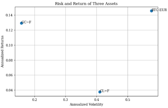
Comparing the Risk and Return of these three assets
plt.figure(figsize=(8,5))
sns.scatterplot(data=table, x="Annualized Volatility", y="Annualized Returns", legend="auto",s=100)
plt.title('Risk and Return of Three Assets')
plt.text(x=table.iloc[0]['Annualized Volatility'],y=table.iloc[0]['Annualized Returns'],s="BTC-EUR")
plt.text(x=table.iloc[1]['Annualized Volatility'],y=table.iloc[1]['Annualized Returns'],s="GC=F")
plt.text(x=table.iloc[2]['Annualized Volatility'],y=table.iloc[2]['Annualized Returns'],s="CL=F")
plt.grid()
plt.show()
Risk and Return of our three assets
This plot shows that BTC gives the highest return, but also highest risk, the Gold asset comes in second with the lowest risk and the Oil asset give the lowest return with the highest volatility.
Covariance vs Correlation Coefficient
Calculating the covariance and correlation coefficient of annualized returns
Running the Scipy SLSQP optimization of portfolio weights with constraints and bounds. The Sharpe ratio’s negative value is minimized in order to derive at the maximum value and the optimal portfolio composition. The constraint is that all parameters (weights) add up to 1. Weights are bound to be between 0 and 1.
Final Comparison: efficient frontier, tangency and minimum variance portfolios.
The solid line represents the optimal portfolios for a particular target return, while the dots represent random portfolios. Furthermore, the figure depicts two larger stars, one for the minimum volatility/variance portfolio (red star symbol) and the other for the portfolio with the maximum Sharpe ratio (yellow star symbol).
Conclusions
The portfolio Bitcoin, Gold, and Oil is highly volatile. Almost all the budget is spent on the Gold instrument.
The maximum Sharpe ratio of 0.83 is not acceptable. Usually, any Sharpe ratio greater than 1.0 is considered acceptable to good by investors. This means we are not being compensated very well for the risk we have taken on.
The proposed portfolio has diversification capabilities that do not complement each other.
However, gold and stocks are driven by separate factors. If an investment portfolio is very heavily inclined toward one asset class or industry, then buying gold might be something to consider.