
Value at Risk (VaR) and Its Implementation in Python

Value at Risk (VaR) is a statistical technique used to measure the risk of loss on a specific portfolio of financial assets. This post will provide a comprehensive understanding of VaR, its importance in risk management, and a practical implementation using Python. We’ll also walk through a detailed example to illustrate how VaR can be calculated and interpreted.
1. What is Value at Risk (VaR)?
Value at Risk (VaR) quantifies the potential loss in value of a portfolio over a defined period for a given confidence interval. For instance, a one-day VaR at a 95% confidence level indicates that there is a 95% chance that the portfolio will not lose more than the VaR amount in one day.
Mathematically, VaR can be expressed as: VaR𝛼(𝑋)=−inf{𝑥∈𝑅∣𝑃(𝑋≤𝑥)>𝛼}VaRα(X)=−inf{x∈R∣P(X≤x)>α} where 𝛼α is the confidence level and 𝑋X is the return distribution of the portfolio.
2. Why is VaR Important?
VaR is a critical tool in risk management for financial institutions and investors because it:
- Provides a clear metric for potential losses.
- Helps in setting risk limits and capital reserves.
- Aids in regulatory compliance and risk reporting.
- Facilitates communication of risk to stakeholders.
Regulatory bodies such as the Basel Committee on Banking Supervision require financial institutions to report their VaR, ensuring that they maintain adequate capital reserves to cover potential losses.
3. Methods to Calculate VaR
There are three primary methods to calculate VaR:
- Historical Method
This method uses historical returns to estimate the potential loss. It involves sorting the historical returns and finding the percentile that corresponds to the desired confidence level.
- Variance-Covariance Method
This method assumes that asset returns are normally distributed. It uses the mean and standard deviation of the portfolio’s returns to calculate VaR. This method is also known as the parametric method.
- Monte Carlo Simulation
This method uses random sampling to simulate a range of potential outcomes based on historical data. It is computationally intensive but flexible in modeling complex portfolios.
4. Implementing VaR in Python
Let’s dive into the implementation of VaR using Python, focusing on each method with a practical example and visualizations.
Historical Method Example
import numpy as np
import pandas as pd
import yfinance as yf
import matplotlib.pyplot as plt

# Fetch historical data for a stock
data = yf.download("AAPL", start="2020-01-01", end="2023-01-01")
returns = data['Adj Close'].pct_change().dropna()

# Calculate the historical VaR at 95% confidence level
confidence_level = 0.95
VaR_historical = np.percentile(returns, (1 - confidence_level) * 100)

print(f"Historical VaR (95% confidence level): {VaR_historical:.2%}")

# Plot the historical returns and VaR threshold
plt.figure(figsize=(10, 6))
plt.hist(returns, bins=50, alpha=0.75, color='blue', edgecolor='black')
plt.axvline(VaR_historical, color='red', linestyle='--', label=f'VaR (95%): {VaR_historical:.2%}')
plt.title('Historical Returns of AAPL')
plt.xlabel('Returns')
plt.ylabel('Frequency')
plt.legend()
plt.show()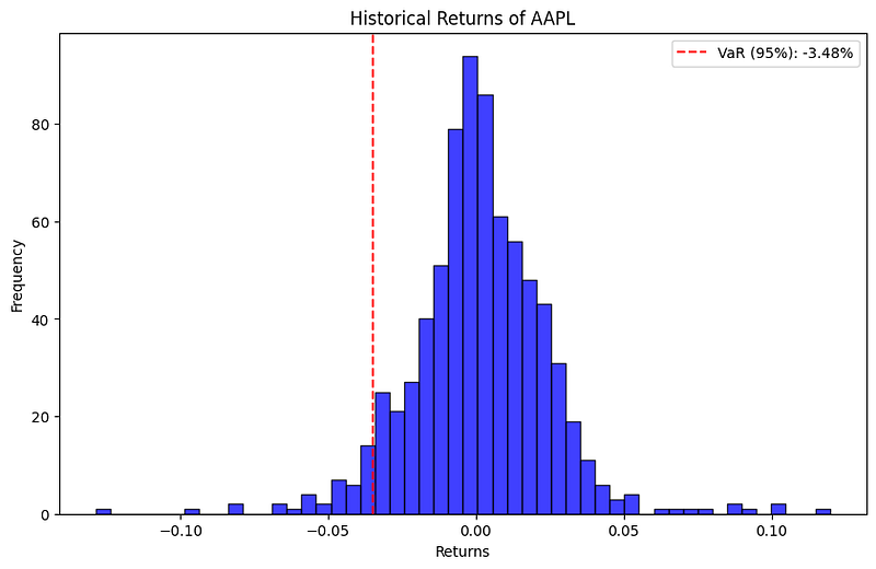
In this example, we use the historical returns of Apple Inc. (AAPL) to calculate the VaR. The histogram displays the distribution of historical returns, and the red dashed line represents the VaR threshold at a 95% confidence level. This visual helps in understanding where the potential losses lie in the distribution of past returns.
Variance-Covariance Method Example
import numpy as np
import yfinance as yf
import matplotlib.pyplot as plt
from scipy.stats import norm

# Fetch historical data for a stock
data = yf.download("AAPL", start="2020-01-01", end="2023-01-01")
returns = data['Adj Close'].pct_change().dropna()

# Calculate the mean and standard deviation of returns
mean_return = np.mean(returns)
std_dev = np.std(returns)

# Calculate the VaR at 95% confidence level using the Z-score
confidence_level = 0.95
z_score = norm.ppf(1 - confidence_level)
VaR_variance_covariance = mean_return + z_score * std_dev

print(f"Variance-Covariance VaR (95% confidence level): {VaR_variance_covariance:.2%}")

# Plot the normal distribution and VaR threshold
plt.figure(figsize=(10, 6))
x = np.linspace(mean_return - 3*std_dev, mean_return + 3*std_dev, 1000)
y = norm.pdf(x, mean_return, std_dev)
plt.plot(x, y, label='Normal Distribution')
plt.axvline(VaR_variance_covariance, color='red', linestyle='--', label=f'VaR (95%): {VaR_variance_covariance:.2%}')
plt.fill_between(x, 0, y, where=(x <= VaR_variance_covariance), color='red', alpha=0.5)
plt.title('Normal Distribution of Returns with VaR Threshold')
plt.xlabel('Returns')
plt.ylabel('Probability Density')
plt.legend()
plt.show()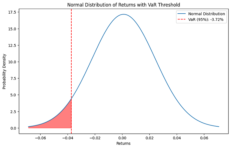
This example uses the variance-covariance method to calculate VaR. The graph illustrates a normal distribution of returns with the VaR threshold marked by a red dashed line. The shaded area under the curve to the left of the VaR threshold represents the probability of losses exceeding the VaR at a 95% confidence level.
Monte Carlo Simulation Example
import numpy as np
import yfinance as yf
import matplotlib.pyplot as plt

# Fetch historical data for a stock
data = yf.download("AAPL", start="2020-01-01", end="2023-01-01")
returns = data['Adj Close'].pct_change().dropna()

# Simulate future returns using Monte Carlo
num_simulations = 10000
simulation_horizon = 252  # Number of trading days in a year
simulated_returns = np.random.normal(np.mean(returns), np.std(returns), (simulation_horizon, num_simulations))

# Calculate the simulated portfolio values
initial_investment = 1000000  # $1,000,000
portfolio_values = initial_investment * np.exp(np.cumsum(simulated_returns, axis=0))

# Calculate the portfolio returns
portfolio_returns = portfolio_values[-1] / portfolio_values[0] - 1

# Calculate the VaR at 95% confidence level
confidence_level = 0.95
VaR_monte_carlo = np.percentile(portfolio_returns, (1 - confidence_level) * 100)

print(f"Monte Carlo VaR (95% confidence level): {VaR_monte_carlo:.2%}")

# Plot the distribution of simulated portfolio returns and VaR threshold
plt.figure(figsize=(10, 6))
plt.hist(portfolio_returns, bins=50, alpha=0.75, color='blue', edgecolor='black')
plt.axvline(VaR_monte_carlo, color='red', linestyle='--', label=f'VaR (95%): {VaR_monte_carlo:.2%}')
plt.title('Simulated Portfolio Returns Distribution')
plt.xlabel('Returns')
plt.ylabel('Frequency')
plt.legend()
plt.show()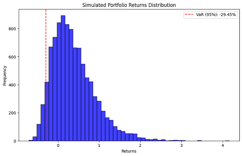
The Monte Carlo simulation example involves generating random returns based on the historical mean and standard deviation. The histogram shows the distribution of simulated portfolio returns, with the VaR threshold at the 95% confidence level marked by a red dashed line. This visualization helps to understand the potential range of future returns and the likelihood of exceeding the VaR.
Value at Risk (VaR) is a vital metric for assessing financial risk, offering a clear quantification of potential losses. By implementing VaR using Python, investors and risk managers can gain actionable insights into their portfolio’s risk profile. The examples provided using the historical method, variance-covariance method, and Monte Carlo simulation demonstrate how versatile and powerful VaR can be in financial risk management.
By understanding and applying these methods, you can enhance your risk management strategies and better safeguard your investments.
If you are interested in more advanced and exclusive content related to Python and Finance topics, you might want to check my Substack newsletter: https://quantitativepy.substack.com/
What To Read Next:
https://quantitativepy.substack.com/p/what-is-a-minimum-variance-portfolio
https://quantitativepy.substack.com/p/mastering-market-trends-with-python


