Is Your Sharpe Ratio Lying to You? Meet the Probabilistic Sharpe Ratio

“Although skewness and kurtosis does not affect the point estimate of Sharpe ratio, it greatly impacts its confidence bands, and consequently its statistical significance” Bailey and López de Prado¹

0. Introduction

In the last article we explained the downfalls of relying on the Central Limit Theorem (CLT) and using the mean and standard deviation to calculate a point estimate of the Sharpe Ratio.

Today, we’ll again be disussing the revered Sharpe Ratio (SR), the metric that has been widely used for decades to measure investment performance relative to risk.

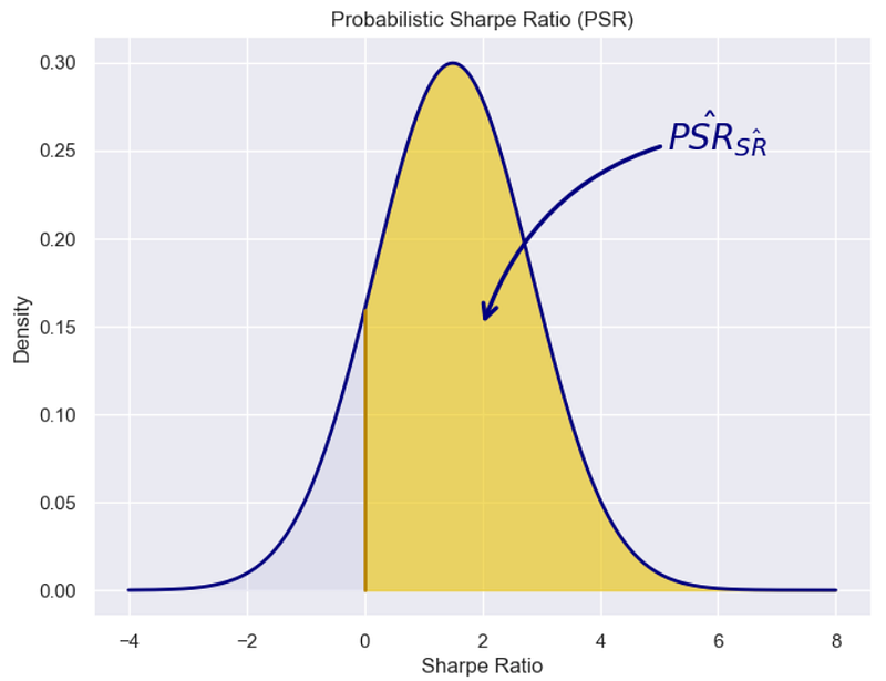
But as with any tried-and-true method, it’s crucial to question its efficacy and explore innovative alternatives. That’s where the Probabilistic Sharpe Ratio (PSR), developed by Bailey and López de Prado, comes into play¹.

What You’ll Learn:

• Understand the Sharpe Ratios limitations
• The basics of PSR and why you should use it
• Python code implementation of PSR
• How to do a “more fair” comparison of Investment Funds SR

Why You Should Read:

• Better risk assessment
• Portfolio optimization
• Make better and more informed decisions

In this article, we’ll delve into the limitations of the Sharpe Ratio, introduce you to the concept of PSR, and guide you through its Python implementation. So if you’re eager to enhance your understanding of risk and performance metrics, you’re in the right place.

1. Limitations of Sharpe Ratio

The Sharpe Ratio has long been the go-to metric for evaluating investment performance relative to risk. However, it’s far from perfect and comes with its own set of limitations.

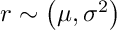
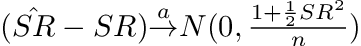
If a strategy has excess returns (risk premium) and returns (r) are independent and identically distributed (IID), where N represents the normal distribution with mean (mu) and variance (sigma²).

As first introduced by Sharpe, a point estimate of the Sharpe Ratio (SR hat) can be evaluated as⁸:

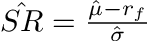
Point Estimate

Maybe the biggest downside of the Sharpe Ratio, is that it is a point estimate, and assumes the Central Limit Theorem (CLT). Hogg and Tanis reported that the CLT generally can be applied for samples in excess of 30 observations³.

Regardless of the number of data points used in order to estimate the Sharpe Ratio, the main issue is that the point estimate does not tell us anything about how likelihood that the portfolio true distrbution does indeed outperform a specific benchmark.

Assumes Normal Distribution

One of the fundamental assumptions of the Sharpe Ratio is that investment returns are normally distributed. This is often not the case, especially for hedge funds and alternative investments.

Non-normal distributions can have skewness and kurtosis, which the point estimate of Sharpe Ratio completely ignores. This is important when conducting hypothesis testing and looking for statistical significance between strategy returns.

Inadequate for Non-linear Strategies

The Sharpe Ratio is primarily designed for portfolios where the risk-return relationship is linear. Hedge funds often employ non-linear strategies that can result in asymmetric risk profiles. This makes the Sharpe Ratio less reliable for such investment approaches.

Penalizes Upside Volatility

The Sharpe Ratio penalizes all volatility, not distinguishing between upside and downside. For many investors, upside volatility is not only acceptable but desired.

This limitation can lead to underestimating the attractiveness of certain strategies. An alternative metric may be The Sortino Ratio but this is outside of the topic of conversation today.

Sensitive to Time Frame

The Sharpe Ratio is sensitive to the time frame of the data used for its calculation. Using daily, monthly, or yearly returns can yield vastly different results.This sensitivity makes it tricky to compare strategies with different investment horizons.

Summary

Limitations of the Sharpe Ratio metric:

• Point estimate of portfolio returns.
• Assumes normal distribution of returns.
• Inadequate for non-linear strategies.
• Penalizes all forms of volatility.
• Sensitive to the chosen time frame.

While the Sharpe Ratio offers a simplified way to assess risk and reward, it is essential to recognize its limitations. This sets the stage for alternative metrics like the Probabilistic Sharpe Ratio (PSR), which addresses many of these issues.

2.0 Introduction to Probabilistic Sharpe Ratio (PSR)

In the world of quantitative finance, evaluating the efficiency of an investment strategy is key. While the Sharpe Ratio has been the go-to metric for many, it has notable limitations. Enter the Probabilistic Sharpe Ratio (PSR), a cutting-edge alternative developed by Marcos López de Prado and David Bailey¹.

Assuming IID Normal Returns

Lo published in The Statistics of Sharpe Ratios assuming independent and identically distributed (IID) Normal returns with skew of 0 and kurtosis of 3, the estimated Sharpe Ratio would follow a normal distribution with standard deviation⁴:

The PSR incorporates skewness and kurtosis into its formulation, two critical statistical moments ignored by the Sharpe Ratio. Here’s where it gets even more interesting: despite these higher-order moments, the PSR distribution can still be assumed to be normal.

Mertens⁵, Christie² and Opdyke⁶ published papers describing the asympototic statistical distribution for the Sharpe Ratio estimate (SR hat). They relaxed the assumptions of normality and independence associated with an unobservable return generating process and only enforced the general assumptions of stationarity (process is time-invariant) and ergodicity (average outcome of a group is the same average outcome for an individual).

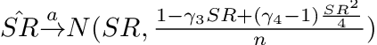
Martens showed that one could drop the normality assumption on returns and yet the estimated Sharpe Ratio would still follow a normal distribution⁵. Christie also showed the Sharpe Ratio estimation by further relaxing assumptions and allowed for returns to have serial correlation, non-IID and time-varying conditional volatilities by using a Gaussian Mixture Model (GMM) approach to derive the limiting distribution². Opdyke⁶ proved that both Martens and Christie’s findings are in fact identical¹.

Ok, but tell me why this matters?

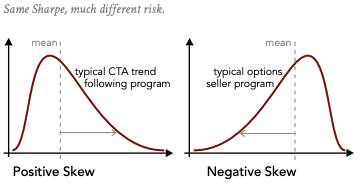
Well, this means that although the Sharpe Ratio follows a normal distribution even if returns do not, combinations of skewness and kurtosis in returns distribution DO IMPACT the standard deviation of the Sharpe Ratio estimate. Below is a graph showing the impact of portfolio returns distributions with skew and kurtosis and the corresponding impact in the standard deviation of the Sharpe Ratio estimate.

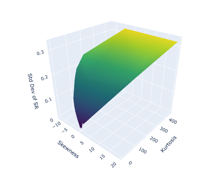
Therefore the skewness and kurtosis of a returns distribution absolutely matters and impacts the confidence bands of the Sharpe Ratio estimate¹. As Bailey and López de Prado suggest, this should be front of mind for a risk-adverse investor.

Building upon this, Bailey and López de Prado’s PSR advances the field by integrating skewness and kurtosis into the formula for the Sharpe Ratio metric, thereby providing a more complete and nuanced picture of an investment’s risk profile¹.

In the next sections, we’ll dive into the mathematical derivation of PSR and its implementation in Python, equipping you with the tools to adopt this advanced metric.

3.0 Sharpe Ratio Confidence Intervals

“Although skewness and kurtosis do not affect the point estimate of the Sharpe ratio, they greatly impact its confidence bands, and consequently its statistical significance”

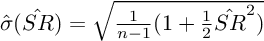
Ok, so we know skew and kurtosis impact our standard deviation of the Sharpe Ratio, but by how much? Because the distribution around the estimate of the Sharpe Ratio is found to follow the normal distribution with variance as described in the previous section, we arrive at the following estimate standard deviation around our Sharpe Ratio estimate¹.

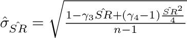
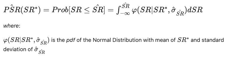
Thanks to its asymptotic statistical distribution, we can construct confidence intervals for the estimated Sharpe Ratio.

This statement describes that the True Sharpe Ratio (SR) is bounded by our estimate (SR hat) with a significance level (alpha). These intervals can be two-sided, lower one-sided, or upper one-sided, and they’re detailed below.

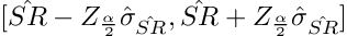
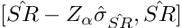
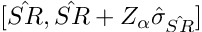
Where Z is the critical value from the standard normal distribution and sigma hat is the standard error of the estimate of SR.

Python Example: Confidence Intervals

from scipy.stats import norm

# Estimated Sharpe Ratio (SR) and number of observations (N)
SR_hat = 1
N = 8

# Calculate Standard Deviation of Sharpe Ratio (Std Dev SR)
def standard_deviation_sharpe_ratio(sharpe_ratio, num_obs, skewness=0, kurtosis=3):
    """Estimates standard Deviation of Sharpe Ratio
    
    Parameters:
    - sharpe_ratio: Sharpe ratio of the strategy
    - bench_sharpe_ratio: Sharpe ratio of the benchmark
    - num_obs: Number of observations
    - skewness: Skewness of the strategy returns (default 0)
    - kurtosis: Kurtosis of the strategy returns (default 3)
    
    Returns:
    - std_dev: Standard Deviation of Sharpe Ratio
    """
    return np.sqrt(
        (1 - skewness*sharpe_ratio + 
         (kurtosis-1)/4*sharpe_ratio**2
        ) / (num_obs-1)
    )

# Portfolio Returns with Normality
sigma_hat_normal_returns = standard_deviation_sharpe_ratio(sharpe_ratio=SR_hat, 
                                                           num_obs=N, 
                                                           skewness=0, 
                                                           kurtosis=3)

# Portfolio Returns with Non-Normality
sigma_hat_higher_moments = standard_deviation_sharpe_ratio(sharpe_ratio=SR_hat, 
                                                           num_obs=N, 
                                                           skewness=-3.5, 
                                                           kurtosis=10)

def two_sided_confidence_intervals(sharpe_ratio, standard_deviation, confidence_level):
    """Sharpe Ratio two-sided confidence intervals

    Parameters:
    - sharpe_ratio: Sharpe ratio of the strategy
    - standard_devation: Standard Deviation of Sharpe Ratio
    - confidence_level: level of confidence (fraction: i.e. 0.90 for 90%)

    Returns:
    - lower_bound: two-sided lower bound
    - upper_bound: two-sided upper bound
    """
    # Two-sided (1-alpha)% Confidence Interval
    alpha = 1 - confidence_level
    Z_alpha_over_2 = norm.ppf(1-alpha/2)  # 95% CI

    lower_bound = sharpe_ratio - Z_alpha_over_2 * standard_deviation
    upper_bound= sharpe_ratio + Z_alpha_over_2 * standard_deviation
    
    return lower_bound, upper_bound

lower_norm, upper_norm = two_sided_confidence_intervals(SR_hat, 
                                                  sigma_hat_normal_returns,
                                                  0.95)

lower_non_norm, upper_non_norm = two_sided_confidence_intervals(SR_hat, 
                                                  sigma_hat_higher_moments,
                                                  0.95)

# Print the confidence intervals
print(f"Normally Distributed; Two-sided 95% CI:     [{lower_norm:2.4f}, {upper_norm:2.4f}]")
print(f"Non-Normally Distributed; Two-sided 95% CI: [{lower_non_norm:2.4f}, {upper_non_norm:2.4f}]")

Constructing these intervals in Python is a breeze, as shown above. These confidence intervals help you gauge the reliability of your Sharpe Ratio estimate. We find when comparing both portfolios with identical Sharpe Ratio of 1, the portfolio with normally distributed returns has much tigher confidence intervals compared to the portfolio with negative skewness and large positive kurtosis at the 95% confidence level.

Normally Distributed; Two-sided 95% CI:     [0.0927, 1.9073]
Non-Normally Distributed; Two-sided 95% CI: [-0.9246, 2.9246]

The higher and lower confidence levels of the non-normally distributed portfolio highlights how skewness and kurtosis with limited number of observations could cause significant inflation of the simple point estimate of the Sharpe Ratio.

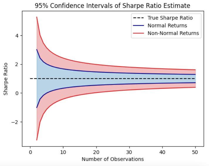
As we can see from the graph, the number of observed returns and the statistical properties of the underlying returns distribution greatly impact the confidence intervals around the Sharpe Ratio estimate.

The main conclusion we would like to draw here, is that Sharpe Ratio estimates are great impacted by these statistical traits:

• Non-normality: skewness and kurtosis
• Reduced granularity: due to returns aggregation

For the risk adverse investor, this example illustrates the importance of considering skewness and kurtosis when using the sharpe ratio for portfolio selection.

4.0 Mathematical Derivation of Probabilistic Sharpe Ratio (PSR)

To fully appreciate the power of the Probabilistic Sharpe Ratio (PSR), let’s delve into its mathematical underpinnings. Recall the formula, as developed by Bailey and López de Prado¹:

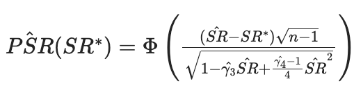
where Φ is the cumulative distribution function of a standard normal distribution, SR is the Sharpe Ratio, SR* is the benchmark Sharpe Ratio, n is the number of observations, and skewness (gamma3) and kurtosis (gamma4) are the third and fourth standardized moments, respectively.

Bailey and López de Prado build on the impressive work Lo⁴, Mertens⁵, Christie² and Opdyke⁶ to create a probabilistic metric based that the distribution of the Sharpe Ratio remains normally distributed even after incorporating skewness and kurtosis.

The integration of skewness and kurtosis elevates PSR beyond traditional metrics. Skewness separates positive outliers from negative ones, adding a layer of risk assessment. Kurtosis measures the fat tails, helping us anticipate extreme market events often ignored by the Sharpe Ratio.

We now possess a more robust tool for risk and performance assessment. The complexity of the formula may seem overwhelming at first, but we will simplify it for you with a Python implementation in the upcoming section.

5.0 Python Tutorial: Implementing Probabilistic Sharpe Ratio (PSR)

Alright, you’ve made it through the theory, now let’s get our hands dirty with some code! In this section, we’ll implement the Probabilistic Sharpe Ratio in Python, giving you a practical tool to add to your quant toolbox.

Requirements:

• Python 3.x
• NumPy
• SciPy

You can install the required packages using pip if you haven’t already:

pip install numpy scipy

Step 1: Import Libraries

import numpy as np
from scipy.stats import norm

Step 2: Define the PSR Function

def probabilistic_sharpe_ratio(sharpe_ratio, bench_sharpe_ratio, num_obs, skewness, kurtosis):
    """
    Calculates the Probabilistic Sharpe Ratio
    
    Parameters:
    - sharpe_ratio: Sharpe ratio of the strategy
    - bench_sharpe_ratio: Sharpe ratio of the benchmark
    - num_obs: Number of observations
    - skewness: Skewness of the strategy returns
    - kurtosis: Kurtosis of the strategy returns
    
    Returns:
    - psr: Probabilistic Sharpe Ratio
    """
    
    sr_diff = sharpe_ratio - bench_sharpe_ratio
    sr_vol = standard_deviation_sharpe_ratio(sharpe_ratio, num_obs, skewness, kurtosis)
    psr = norm.cdf(sr_diff / sr_vol)
    
    return psr

With just a few lines of code, you’ve got a function that calculates the PSR. The function takes in the Sharpe Ratio (SR), the benchmark Sharpe Ratio (SR*), skewness, kurtosis, and the number of observations (N) as parameters.

Step 3: Example Calculation

# Sample data
SR = 0.5  # Your strategy's Sharpe Ratio
Bench_SR = 0.3  # Benchmark Sharpe Ratio
skewness = -0.2  # Skewness of your strategy
kurtosis = 3.5  # Kurtosis of your strategy
N = 252  # Number of observations (trading days in a year, for example)

# Calculate PSR
PSR_value = probabilistic_sharpe_ratio(SR, Bench_SR, N, skewness, kurtosis)
print(f"Probabilistic Sharpe Ratio: {PSR_value}")

After defining the function, I’ve included a sample calculation. Replace the sample data with your own strategy and benchmark metrics to get a personalized PSR value.

By integrating this Python function into your quantitative workflow, you’ll be empowered to assess your investment strategies through the lens of the Probabilistic Sharpe Ratio. This offers a more nuanced and comprehensive view compared to the traditional Sharpe Ratio.

6.0 A Tricky but Realistic Example…

In the graph below there are two portfolio’s with exactly the same True Sharpe Ratio of 1.5:

1. Returns are normally distributed (iid)
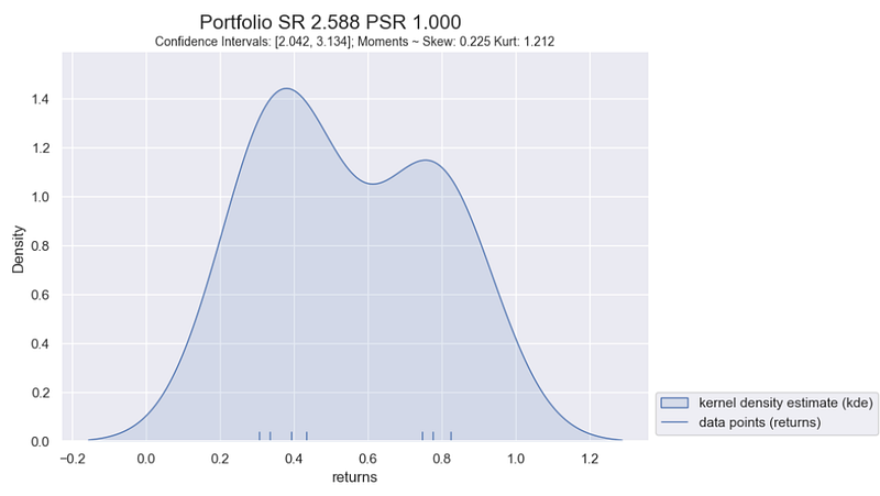
2. Returns are non-normally distributed (iid) with skew of ~ -1.2 and kurtosis of ~5.3

The mixture of two Gaussians can be used to create a distribution with both skew and kurtosis, allowing for a more realistic modeling of financial returns. Below in the chart, gmm (blue distribution), is a gaussian mixture model between two normal distributions with roughly 8% chance of sampling from gaussian 2 and 92% from gaussian 1. The resulting returns distribution has significant non-normal statistical traits, however, it has the exact same Sharpe Ratio of 1.5 as in the normally distributed portfolio in red.

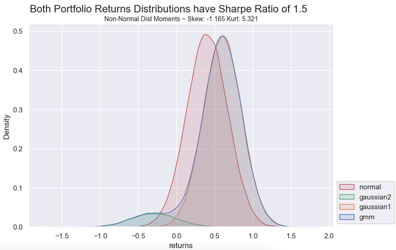
Although both portfolio’s have exactly the same Sharpe Ratio, depending on the number of returns observations we would have very different confidence levels around our estimates.

Let’s say we are considering both portfolio’s and only have 2 years of quarterly returns to estimate the Sharpe Ratio’s. This would be a total of 8 data points. The following code allows us to simulate the portfolio’s from their respective true distributions and visualise the results. The graphs below show estimated:

• Sharpe Ratios,
• Probabilistic Sharpe Ratio,
• Confidence Intervals, and
• Higher Order Moments (skew and kurtosis).

import numpy as np
import scipy as sc
import seaborn as sns
import matplotlib.pyplot as plt

benchmark_sr=0
no_obs=8
means=np.array([0.6, -0.3])
std_devs=np.array([0.25, 0.3])
SR = np.array([1.5])
along_axis = np.hstack((SR, means, std_devs))
probs = generate_p_along_axis(along_axis)

print(f"Probability for GMM is {probs}")

mean=0.4
normal = np.random.normal(loc=mean, scale=mean/1.5, size=no_obs)
gmm1 = generate_gmm_data(means, std_devs, weights=[probs, 1-probs], n_samples=no_obs)

sharpe_ratio0 = np.mean(normal)/np.std(normal)
skew0 = sc.stats.skew(normal)
kurt0 = sc.stats.kurtosis(normal)
psr0 = probabilistic_sharpe_ratio(sharpe_ratio0, benchmark_sr, no_obs, skew0, kurt0+3)
sigma0 = standard_deviation_sharpe_ratio(sharpe_ratio0, no_obs, skew0, kurt0+3)
confinv0 = two_sided_confidence_intervals(sharpe_ratio0, sigma0, 0.95)

sharpe_ratio1 = np.mean(gmm1)/np.std(gmm1)
skew1 = sc.stats.skew(gmm1)
kurt1 = sc.stats.kurtosis(gmm1)
psr1 = probabilistic_sharpe_ratio(sharpe_ratio1, benchmark_sr, no_obs, skew1, kurt1+3)
sigma1 = standard_deviation_sharpe_ratio(sharpe_ratio1, no_obs, skew1, kurt1+3)
confinv1 = two_sided_confidence_intervals(sharpe_ratio1, sigma1, 0.95)

def displot(data, sharpe_ratio, psr, skew, kurtosis, confinv):
    sns.displot([data], kind='kde', fill=True, rug=True, legend=False, alpha=0.15, height=5, aspect=1.5)
    plt.legend(['kernel density estimate (kde)','data points (returns)'], loc='lower left', bbox_to_anchor=(1, 0))
    plt.xlabel('returns')
    plt.suptitle(f'Portfolio SR {sharpe_ratio:2.3f} PSR {psr:2.3f}', y=1.05, fontsize=16)
    plt.title(f'Confidence Intervals: [{confinv[0]:2.3f}, {confinv[1]:2.3f}]; Moments ~ Skew: {skew:2.3f} Kurt: {kurtosis+3:2.3f}', fontsize=10)
    plt.show()

displot(normal, sharpe_ratio0, psr0, skew0, kurt0, confinv0)
displot(gmm1, sharpe_ratio1, psr1, skew1, kurt1, confinv1)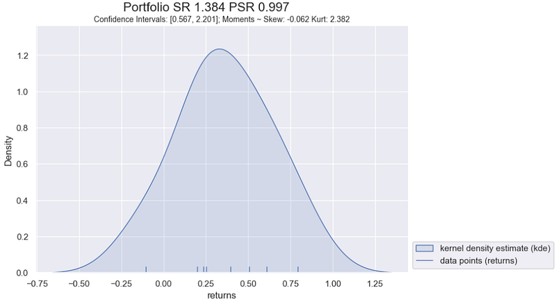

Our first observation — in this particular simulation — is that the normally distributed portfolio after only 8 observed returns has an estimated Sharpe Ratio of 1.38 which is very close to the true Sharpe Ratio of 1.5.

In comparision, for the non-normally distributed portfolio we have an inflated Sharpe Ratio estimate of 2.59. This is primarly due to the low likelihood of downside risk (~8% chance), of having a return from the gaussian 2 part of the distribution. With only 8 data points, our sample does not accurately represent the downside risk of the portfolio and has resulted in an inflated estimate of our Sharpe Ratio and also our Probabilistic Sharpe Ratio value.

This observation natural leads us to think:

“How long should a track record be in order to have statistical confidence that its Sharpe ratio is above a given threshold?” Bailey and López de Prado¹

This is a question we will address in our next article.

7.0 Summary

In this article, we’ve delved into the nuances of Probabilistic Sharpe Ratio (PSR), offering a more comprehensive lens for evaluating portfolio performance. Building upon the original work by Lo⁴, Mertens⁵, Christie² and Opdyke⁶ both Bailey and López de Prado’s created a metric that accounts for the standard deviation and uncertainty associated with estimating Sharpe Ratio even from portfolio’s with true distributions that are non-normally distributed.

Sharpe Ratios are greatly impacting by statistical traits like non-normality and reduced granularity, and therefore Bailey and Lopez de Prado recommend adopting:

1. Probabilistic Sharpe Ratio (PSR): By incorperating the PSR metric into our analysis we are accounting for the non-normal characteristics that can impact statistical significance our Sharpe Ratio estimate. Therefore by using the PSR we can reduce the rate of discovery of false positives (Type I errors).
2. High-Frequency Reporting: For portfolios with undesirable statistical traits, the paper advocates for the highest reporting frequency that doesn’t violate the IID (Independently and Identically Distributed) assumption, enhancing the reliability of the performance metrics.

Bailey and López de Prado also created a frameword to determine the minimum track record length required to have statistical confidence that a Sharpe Ratio is above a given threshold. This is be the topic of discussion in the next article!

References

1. Bailey DH, López de Prado, M. The Sharpe Ratio Efficient Frontier. Journal of Risk. 2012; 15(2). doi: 10.2139/ssrn.1821643
2. Christie S. Is the Sharpe Ratio Useful in Asset Allocation. AFC Research Papers №31, Applied Finance Centre, Macquarie University. 2005. doi: 10.2139/ssrn.720801
3. Hogg R, Tanis E. Probability and Statistical Inference. Pearson. 9th ed. 2013.
4. Lo A. The Statistics of Sharpe Ratios. Financial Analysts Journal. 2002; 58(4): 36–52. doi: 10.2469/faj.v58.n4.2453
5. Mertens E. Variance of the IID estimator in Lo (2002). Working paper, University of Basel. 2002.
6. Opdyke J. Comparing Sharpe ratios: so where are the p-values?. Journal of Asset Management. 2007; 8(5): 308–336. doi: 10.1057/palgrave.jam.2250084
7. Rollinger TN, Hoffman ST. Sortino: A ‘Sharper’ Ratio. Red Rock. 2016. http://www.redrockcapital.com/Sortino__A__Sharper__Ratio_Red_Rock_Capital.pdf
8. Sharpe W. The Sharpe ratio. Journal of Portfolio Management. 1994; 21(1): 49–58. doi: 10.3905/jpm.1994.409501